20. 预测 AR(1) 过程#
!pip install arviz pymc
本讲座介绍了用于预测一元自回归过程未来值函数的统计方法。
这些方法旨在考虑这些统计量的两个可能的不确定性来源:
影响转换规律的随机冲击
AR(1)过程参数值的不确定性
我们考虑两类统计量:
由AR(1)过程控制的随机过程 \(\{y_t\}\)的预期值 \(y_{t+j}\)
在时间 \(t\) 被定义为未来值 \(\{y_{t+j}\}_{j ≥ 1}\) 的非线性函数的样本路径特性
样本路径特性是指诸如”到下一个转折点的时间”或”到下一次衰退的时间”之类的特征。
为研究样本路径特性,我们将使用Wecker [Wecker, 1979]推荐的模拟程序。
为了考虑参数的不确定性,我们将使用pymc构建未知参数的贝叶斯联合后验分布。
让我们从一些导入开始。
import numpy as np
import arviz as az
import pymc as pmc
import matplotlib.pyplot as plt
import matplotlib as mpl
import seaborn as sns

sns.set_style('white')
colors = sns.color_palette()
FONTPATH = "fonts/SourceHanSerifSC-SemiBold.otf"
mpl.font_manager.fontManager.addfont(FONTPATH)
plt.rcParams['font.family'] = ['Source Han Serif SC']

import logging
logging.basicConfig()
logger = logging.getLogger('pymc')
logger.setLevel(logging.CRITICAL)
20.1. 一元一阶自回归过程#
考虑一元AR(1)模型:
其中标量 \(\rho\) 和 \(\sigma\) 满足 \(|\rho| < 1\) 和 \(\sigma > 0\); \(\{\epsilon_{t+1}\}\) 是一个均值为 \(0\)、方差为 \(1\) 的独立同分布正态随机变量序列。
初始条件 \(y_{0}\) 是一个已知数。
方程(20.1)表明对于 \(t \geq 0\),\(y_{t+1}\) 的条件密度为
此外,方程(20.1)还表明对于\(t \geq 0, j \geq 1\),\(y_{t+j}\) 的条件密度为
预测分布(20.3)假设参数 \(\rho, \sigma\) 是已知的,我们通过以它们为条件来表达。
我们还想计算一个不以 \(\rho,\sigma\) 为条件,而是考虑到它们的不确定性的预测分布。
根据一个观测历史 \(y^t = \{y_s\}_{s=0}^t\),我们有联合后验分布 \(\pi_t(\rho,\sigma | y^t)\)。我们通过对 (20.3)关于 \(\pi_t(\rho,\sigma | y^t)\) 进行积分来形成这个预测分布:
预测分布(20.3)假设参数 \((\rho,\sigma)\) 是已知的。
预测分布(20.4)假设参数 \((\rho,\sigma)\) 是不确定的,但有已知的概率分布 \(\pi_t(\rho,\sigma | y^t)\)。
我们还想计算一些”样本路径统计量”的预测分布,这可能包括
到下一次”衰退”的时间,
未来8个周期内 \(Y\) 的最小值,
“严重衰退”,以及
到下一个转折点(正或负)的时间。
为了在我们对参数值不确定的情况下实现这一目标,我们将按以下方式扩展Wecker的[Wecker, 1979]方法。
首先,模拟一个长度为\(T_0\)的初始路径;
对于给定的先验分布,在观察初始路径后从参数 \(\left(\rho,\sigma\right)\) 的后验联合分布中抽取大小为 \(N\) 的样本;
对于每个抽样 \(n=0,1,...,N\),用参数 \(\left(\rho_n,\sigma_n\right)\) 模拟长度为 \(T_1\) 的”未来路径”,并计算我们的三个”样本路径统计量”;
最后,将 \(N\) 个样本的所需统计量绘制为经验分布。
20.2. 实现#
首先,我们将模拟一个样本路径,并以此为基础进行我们的预测。
除了绘制样本路径外,在假设已知真实参数值的情况下,我们将使用上述(20.3)所描述的条件分布绘制 \(.9\) 和 \(.95\) 的覆盖区间。
我们还将绘制一系列未来值序列的样本,并观察它们相对于覆盖区间落在何处。
def AR1_simulate(rho, sigma, y0, T):

    # 分配空间并生成随机误差项
    y = np.empty(T)
    eps = np.random.normal(0, sigma, T)

    # 初始条件并向前推进
    y[0] = y0
    for t in range(1, T):
        y[t] = rho * y[t-1] + eps[t]

    return y


def plot_initial_path(initial_path):
    """
    绘制初始路径和前面的预测密度
    """
    # 计算0.9置信区间
    y0 = initial_path[-1]
    center = np.array([rho**j * y0 for j in range(T1)])
    vars = np.array([sigma**2 * (1 - rho**(2 * j)) / (1 - rho**2) for j in range(T1)])
    y_bounds1_c95, y_bounds2_c95 = center + 1.96 * np.sqrt(vars), center - 1.96 * np.sqrt(vars)
    y_bounds1_c90, y_bounds2_c90 = center + 1.65 * np.sqrt(vars), center - 1.65 * np.sqrt(vars)

    # 绘图
    fig, ax = plt.subplots(1, 1, figsize=(12, 6))
    ax.set_title("初始路径和预测密度", fontsize=15)
    ax.plot(np.arange(-T0 + 1, 1), initial_path)
    ax.set_xlim([-T0, T1])
    ax.axvline(0, linestyle='--', alpha=.4, color='k', lw=1)

    # 模拟未来路径
    for i in range(10):
        y_future = AR1_simulate(rho, sigma, y0, T1)
        ax.plot(np.arange(T1), y_future, color='grey', alpha=.5)

    # 绘制90%置信区间
    ax.fill_between(np.arange(T1), y_bounds1_c95, y_bounds2_c95, alpha=.3, label='95%置信区间')
    ax.fill_between(np.arange(T1), y_bounds1_c90, y_bounds2_c90, alpha=.35, label='90%置信区间')
    ax.plot(np.arange(T1), center, color='red', alpha=.7, label='期望均值')
    ax.legend(fontsize=12)
    plt.show()


sigma =  1
rho = 0.9
T0, T1 = 100, 100
y0 = 10

# 模拟
np.random.seed(145)
initial_path = AR1_simulate(rho, sigma, y0, T0)

# 绘图
plot_initial_path(initial_path)

作为预测期的函数,置信区间的形状类似于 https://python.quantecon.org/perm_income_cons.html 中所描述的。
20.3. 路径属性的预测分布#
Wecker [Wecker, 1979] 提出使用模拟技术来表征某些统计量的预测分布,这些统计量是 \(y\) 的非线性函数。
他将这些函数称为”路径属性”,以区别于单个数据点的属性。
他研究了给定序列 \(\{y_t\}\) 的两个特殊的未来路径属性。
第一个是到下一个转折点的时间。
他将 “转折点” 定义为 \(y\) 连续两次下降中的第二个时间点。
为了研究这个统计量,让 \(Z\) 作为一个指示过程
那么到下一个转折点的时间这个随机变量被定义为关于\(Z\)的以下停时:
Wecker [Wecker, 1979]还研究了未来8个季度 \(Y\) 的最小值,可以定义为随机变量:
研究另一个可能的转折点概念也很有意思。
因此,令
定义今天或明天的正转折点统计量为
这被设计用来表示以下事件:
“在一次或两次下降之后,\(Y\) 将连续两个季度增长”
根据[Wecker, 1979],我们可以通过模拟来计算每个时期 \(t\) 的 \(P_t\) 和 \(N_t\) 的概率。
20.4. 一个类似Wecker的算法#
该过程包含以下步骤:
用 \(\omega_i\) 标记样本路径
对于给定日期 \(t\),模拟 \(I\) 条长度为 \(N\) 的样本路径
对每条路径 \(\omega_i\),计算相应的 \(W_t(\omega_i), W_{t+1}(\omega_i), \dots\) 值
将集合 \(\{W_t(\omega_i)\}^{T}_{i=1}, \ \{W_{t+1}(\omega_i)\}^{T}_{i=1}, \ \dots, \ \{W_{t+N}(\omega_i)\}^{T}_{i=1}\) 视为来自预测分布 \(f(W_{t+1} \mid \mathcal y_t, \dots)\), \(f(W_{t+2} \mid y_t, y_{t-1}, \dots)\), \(\dots\), \(f(W_{t+N} \mid y_t, y_{t-1}, \dots)\) 的样本。
20.5. 使用模拟来近似后验分布#
下面的代码单元使用 pymc 计算时间 \(t\) 时 \(\rho, \sigma\) 的后验分布。
注意在定义似然函数时,我们选择以初始值 \(y_0\) 为条件。
def draw_from_posterior(sample):
    """
    从后验分布中抽取大小为N的样本。
    """

    AR1_model = pmc.Model()

    with AR1_model:

        # 从先验开始
        rho = pmc.Uniform('rho',lower=-1.,upper=1.)  # 假设rho稳定
        sigma = pmc.HalfNormal('sigma', sigma = np.sqrt(10))

        # 下一期y的期望值(rho * y)
        yhat = rho * sample[:-1]

        # 实际实现值的似然
        y_like = pmc.Normal('y_obs', mu=yhat, sigma=sigma, observed=sample[1:])

    with AR1_model:
        trace = pmc.sample(10000, tune=5000)

    # 检查条件
    with AR1_model:
        az.plot_trace(trace, figsize=(17, 6))

    rhos = trace.posterior.rho.values.flatten()
    sigmas = trace.posterior.sigma.values.flatten()

    post_sample = {
        'rho': rhos,
        'sigma': sigmas
    }

    return post_sample

post_samples = draw_from_posterior(initial_path)
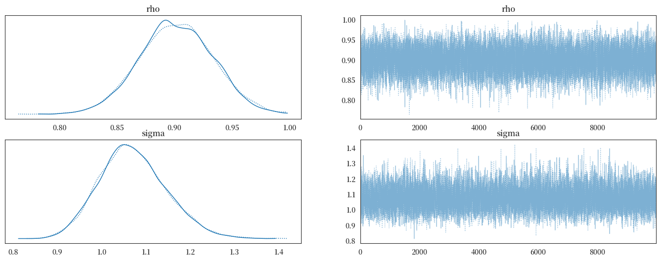
左侧的图表展示了后验边际分布。
20.6. 计算样本路径统计量#
接下来我们准备Python代码来计算我们的样本路径统计量。
# 定义统计量
def next_recession(omega):
    n = omega.shape[0] - 3
    z = np.zeros(n, dtype=int)

    for i in range(n):
        z[i] = int(omega[i] <= omega[i+1] and omega[i+1] > omega[i+2] and omega[i+2] > omega[i+3])

    if np.any(z) == False:
        return 500
    else:
        return np.where(z==1)[0][0] + 1

def minimum_value(omega):
    return min(omega[:8])

def severe_recession(omega):
    z = np.diff(omega)
    n = z.shape[0]

    sr = (z < -.02).astype(int)
    indices = np.where(sr == 1)[0]

    if len(indices) == 0:
        return T1
    else:
        return indices[0] + 1

def next_turning_point(omega):
    """
    假设omega的长度为6

        y_{t-2}, y_{t-1}, y_{t}, y_{t+1}, y_{t+2}, y_{t+3}

    这足以确定P/N的值
    """

    n = np.asarray(omega).shape[0] - 4
    T = np.zeros(n, dtype=int)

    for i in range(n):
        if ((omega[i] > omega[i+1]) and (omega[i+1] > omega[i+2]) and
            (omega[i+2] < omega[i+3]) and (omega[i+3] < omega[i+4])):
            T[i] = 1
        elif ((omega[i] < omega[i+1]) and (omega[i+1] < omega[i+2]) and
            (omega[i+2] > omega[i+3]) and (omega[i+3] > omega[i+4])):
            T[i] = -1

    up_turn = np.where(T == 1)[0][0] + 1 if (1 in T) == True else T1
    down_turn = np.where(T == -1)[0][0] + 1 if (-1 in T) == True else T1

    return up_turn, down_turn
20.7. 原始Wecker方法#
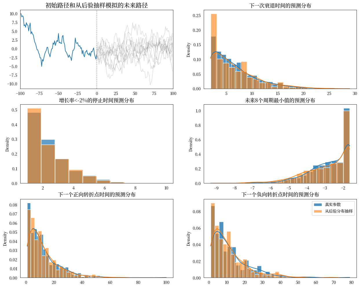
现在我们应用Wecker的原始方法,以与数据生成模型相关的真实参数为条件,通过模拟未来路径并计算预测分布。
def plot_Wecker(initial_path, N, ax):
    """
    绘制"纯"韦克方法的预测分布。
    """
    # 存储结果
    next_reces = np.zeros(N)
    severe_rec = np.zeros(N)
    min_vals = np.zeros(N)
    next_up_turn, next_down_turn = np.zeros(N), np.zeros(N)

    # 计算0.9置信区间
    y0 = initial_path[-1]
    center = np.array([rho**j * y0 for j in range(T1)])
    vars = np.array([sigma**2 * (1 - rho**(2 * j)) / (1 - rho**2) for j in range(T1)])
    y_bounds1_c95, y_bounds2_c95 = center + 1.96 * np.sqrt(vars), center - 1.96 * np.sqrt(vars)
    y_bounds1_c90, y_bounds2_c90 = center + 1.65 * np.sqrt(vars), center - 1.65 * np.sqrt(vars)

    # 绘图
    ax[0, 0].set_title("初始路径和预测密度", fontsize=15)
    ax[0, 0].plot(np.arange(-T0 + 1, 1), initial_path)
    ax[0, 0].set_xlim([-T0, T1])
    ax[0, 0].axvline(0, linestyle='--', alpha=.4, color='k', lw=1)

    # 绘制90%置信区间
    ax[0, 0].fill_between(np.arange(T1), y_bounds1_c95, y_bounds2_c95, alpha=.3)
    ax[0, 0].fill_between(np.arange(T1), y_bounds1_c90, y_bounds2_c90, alpha=.35)
    ax[0, 0].plot(np.arange(T1), center, color='red', alpha=.7)

    # 模拟未来路径
    for n in range(N):
        sim_path = AR1_simulate(rho, sigma, initial_path[-1], T1)
        next_reces[n] = next_recession(np.hstack([initial_path[-3:-1], sim_path]))
        severe_rec[n] = severe_recession(sim_path)
        min_vals[n] = minimum_value(sim_path)
        next_up_turn[n], next_down_turn[n] = next_turning_point(sim_path)

        if n%(N/10) == 0:
            ax[0, 0].plot(np.arange(T1), sim_path, color='gray', alpha=.3, lw=1)

    # 返回next_up_turn, next_down_turn
    sns.histplot(next_reces, kde=True, stat='density', ax=ax[0, 1], alpha=.8, label='真实参数')
    ax[0, 1].set_title("下一次衰退时间的预测分布", fontsize=13)

    sns.histplot(severe_rec, kde=False, stat='density', ax=ax[1, 0], binwidth=0.9, alpha=.7, label='真实参数')
    ax[1, 0].set_title(r"增长率<-2%的停止时间预测分布", fontsize=13)

    sns.histplot(min_vals, kde=True, stat='density', ax=ax[1, 1], alpha=.8, label='真实参数')
    ax[1, 1].set_title("未来8个周期最小值的预测分布", fontsize=13)

    sns.histplot(next_up_turn, kde=True, stat='density', ax=ax[2, 0], alpha=.8, label='真实参数')
    ax[2, 0].set_title("下一个正向转折点时间的预测分布", fontsize=13)

    sns.histplot(next_down_turn, kde=True, stat='density', ax=ax[2, 1], alpha=.8, label='真实参数')
    ax[2, 1].set_title("下一个负向转折点时间的预测分布", fontsize=13)

fig, ax = plt.subplots(3, 2, figsize=(15,12))
plot_Wecker(initial_path, 1000, ax)
plt.show()

20.8. 扩展 Wecker 方法#
现在,我们应用我们的的”扩展” Wecker 方法。该方法基于 (20.4) 定义的 \(y\) 的预测密度,考虑了参数 \(\rho, \sigma\) 的后验不确定性。
为了近似 (20.4) 右侧的积分,我们每次从模型 (20.1) 中模拟未来值序列时,都重复地从联合后验分布中抽取参数。
def plot_extended_Wecker(post_samples, initial_path, N, ax):
    """
    绘制扩展 Wecker 的预测分布
    """
    # 选择样本
    index = np.random.choice(np.arange(len(post_samples['rho'])), N + 1, replace=False)
    rho_sample = post_samples['rho'][index]
    sigma_sample = post_samples['sigma'][index]

    # 存储结果
    next_reces = np.zeros(N)
    severe_rec = np.zeros(N)
    min_vals = np.zeros(N)
    next_up_turn, next_down_turn = np.zeros(N), np.zeros(N)

    # 绘图
    ax[0, 0].set_title("初始路径和从后验抽样模拟的未来路径", fontsize=15)
    ax[0, 0].plot(np.arange(-T0 + 1, 1), initial_path)
    ax[0, 0].set_xlim([-T0, T1])
    ax[0, 0].axvline(0, linestyle='--', alpha=.4, color='k', lw=1)

    # 模拟未来路径
    for n in range(N):
        sim_path = AR1_simulate(rho_sample[n], sigma_sample[n], initial_path[-1], T1)
        next_reces[n] = next_recession(np.hstack([initial_path[-3:-1], sim_path]))
        severe_rec[n] = severe_recession(sim_path)
        min_vals[n] = minimum_value(sim_path)
        next_up_turn[n], next_down_turn[n] = next_turning_point(sim_path)

        if n % (N / 10) == 0:
            ax[0, 0].plot(np.arange(T1), sim_path, color='gray', alpha=.3, lw=1)

    # 返回 next_up_turn, next_down_turn
    sns.histplot(next_reces, kde=True, stat='density', ax=ax[0, 1], alpha=.6, color=colors[1], label='从后验分布抽样')
    ax[0, 1].set_title("下一次衰退时间的预测分布", fontsize=13)

    sns.histplot(severe_rec, kde=False, stat='density', ax=ax[1, 0], binwidth=.9, alpha=.6, color=colors[1], label='从后验分布抽样')
    ax[1, 0].set_title(r"增长率<-2%的停止时间预测分布", fontsize=13)

    sns.histplot(min_vals, kde=True, stat='density', ax=ax[1, 1], alpha=.6, color=colors[1], label='从后验分布抽样')
    ax[1, 1].set_title("未来8个周期最小值的预测分布", fontsize=13)

    sns.histplot(next_up_turn, kde=True, stat='density', ax=ax[2, 0], alpha=.6, color=colors[1], label='从后验分布抽样')
    ax[2, 0].set_title("下一个正向转折点时间的预测分布", fontsize=13)

    sns.histplot(next_down_turn, kde=True, stat='density', ax=ax[2, 1], alpha=.6, color=colors[1], label='从后验分布抽样')
    ax[2, 1].set_title("下一个负向转折点时间的预测分布", fontsize=13)

fig, ax = plt.subplots(3, 2, figsize=(15, 12))
plot_extended_Wecker(post_samples, initial_path, 1000, ax)
plt.show()

20.9. 比较#
最后,我们将原始的Wecker方法和从后验分布中抽取参数值的扩展方法一起绘制,以比较在参数实际不确定时假装知道参数值所产生的差异。
fig, ax = plt.subplots(3, 2, figsize=(15,12))
plot_Wecker(initial_path, 1000, ax)
ax[0, 0].clear()
plot_extended_Wecker(post_samples, initial_path, 1000, ax)
plt.legend()
plt.show()