45. 工作搜寻 IV:相关工资报价#
除了Anaconda中的内容外,本讲座还需要以下库:
!pip install quantecon
45.1. 概述#
在本讲座中,我们求解一个工资报价由持续性和暂时性成分组成的McCall工作搜寻模型。
换句话说,我们放宽了工资随机性在时间上独立的假设。
同时,我们将回到假设工作是永久性的,不会发生离职。
这是为了在研究相关性影响时保持模型相对简单。
我们将使用以下导入:
import matplotlib.pyplot as plt
import matplotlib as mpl
FONTPATH = "fonts/SourceHanSerifSC-SemiBold.otf"
mpl.font_manager.fontManager.addfont(FONTPATH)
plt.rcParams['font.family'] = ['Source Han Serif SC']

import numpy as np
import quantecon as qe
from numpy.random import randn
from numba import jit, prange, float64
from numba.experimental import jitclass
45.2. 模型#
每个时期的工资由下式给出:
其中
这里 \(\{ \zeta_t \}\) 和 \(\{ \epsilon_t \}\) 都是独立同分布的标准正态随机变量。
这里 \(\{y_t\}\) 是暂时性成分,\(\{z_t\}\) 是持续性成分。
如前所述,劳动者可以:
接受当前工作机会,并在该工资水平永久工作,或
领取失业补偿金 \(c\) 并等待下一期。
价值函数满足贝尔曼方程:
在这个表达式中,\(u\) 是效用函数,\(\mathbb E_z\) 是给定当前 \(z\) 时下一期变量的条件期望。
变量 \(z\) 作为状态变量进入贝尔曼方程,这是因为它的当前值有助于预测未来工资。
45.2.1. 简化#
我们可以通过以下方法降低问题维度,显著提升计算效率:
首先,让 \(f^*\) 为延续价值函数,定义为:
现在贝尔曼方程可以写成:
结合上述两个表达式,我们看到延续价值函数满足:
为求解该函数方程,我们引入算子\(Q\):
根据构造,\(f^*\) 是 \(Q\) 的不动点,即 \(Q f^* = f^*\)。
在较弱的假设下,可以证明 \(Q\) 是 \(\mathbb R\) 上连续函数空间上的一个压缩映射。
根据巴拿赫压缩映射定理,\(f^*\) 是唯一的不动点,我们可以从任何合理的初始条件开始通过迭代 \(Q\) 来得到\(f^*\)。
求得 \(f^*\)后,这一搜索问题的解就是当接受工作的收益超过延续价值时停止求职,即:
对于效用函数,我们取 \(u(c) = \ln(c)\)。
保留工资是最后一个表达式中等式成立的工资:
我们的主要目标是求解该保留工资规则,并分析其性质与含义。
45.3. 实现#
让 \(f\) 作为我们对 \(f^*\) 的初始猜测。
在迭代时,我们使用拟合价值函数迭代算法。
特别地,\(f\) 和所有后续迭代值都作为向量存储在一个网格。
这些点通过分段线性插值转换为函数。
\(Qf\) 定义中的期望项通过蒙特卡洛计算。
以下类型声明帮助 Numba 进行类型推断:
job_search_data = [
     ('μ', float64),             # 暂时性冲击对数均值
     ('s', float64),             # 暂时性冲击对数方差
     ('d', float64),             # 持续性状态位移系数
     ('ρ', float64),             # 持续性状态相关系数
     ('σ', float64),             # 状态波动率
     ('β', float64),             # 折现因子
     ('c', float64),             # 失业补助
     ('z_grid', float64[:]),     # 状态空间网格
     ('e_draws', float64[:,:])   # 积分用的蒙特卡洛抽取
]
这是一个存储数据和贝尔曼方程右侧项的类。
默认参数值嵌入在类中。
@jitclass(job_search_data)
class JobSearch:

    def __init__(self,
                 μ=0.0,       # 暂时性冲击对数均值
                 s=1.0,       # 暂时性冲击对数方差
                 d=0.0,       # 持续性状态位移系数
                 ρ=0.9,       # 持续性状态相关系数
                 σ=0.1,       # 状态波动率
                 β=0.98,      # 折现因子
                 c=5,         # 失业补助
                 mc_size=1000,
                 grid_size=100):

        self.μ, self.s, self.d,  = μ, s, d,
        self.ρ, self.σ, self.β, self.c = ρ, σ, β, c

        # 设置网格
        z_mean = d / (1 - ρ)
        z_sd = σ / np.sqrt(1 - ρ**2)
        k = 3  # 标准差倍数
        a, b = z_mean - k * z_sd, z_mean + k * z_sd
        self.z_grid = np.linspace(a, b, grid_size)

        # 生成并存储冲击
        np.random.seed(1234)
        self.e_draws = randn(2, mc_size)

    def parameters(self):
        """
        返回所有参数作为元组。
        """
        return self.μ, self.s, self.d, \
                self.ρ, self.σ, self.β, self.c
接下来我们实现 \(Q\) 算子。
@jit(parallel=True)
def Q(js, f_in, f_out):
    """
    应用算子Q。

        * js 是 JobSearch 的实例
        * f_in 和 f_out 是表示 f 和 Qf 的数组

    """

    μ, s, d, ρ, σ, β, c = js.parameters()
    M = js.e_draws.shape[1]

    for i in prange(len(js.z_grid)):
        z = js.z_grid[i]
        expectation = 0.0
        for m in range(M):
            e1, e2 = js.e_draws[:, m]
            z_next = d + ρ * z + σ * e1
            go_val = np.interp(z_next, js.z_grid, f_in)  # f(z')
            y_next = np.exp(μ + s * e2)                  # 生成 y'
            w_next = np.exp(z_next) + y_next             # 生成 w'
            stop_val = np.log(w_next) / (1 - β)
            expectation += max(stop_val, go_val)
        expectation = expectation / M
        f_out[i] = np.log(c) + β * expectation
这是一个计算 \(Q\) 不动点近似值的函数。
def compute_fixed_point(js,
                        use_parallel=True,
                        tol=1e-4,
                        max_iter=1000,
                        verbose=True,
                        print_skip=25):

    f_init = np.full(len(js.z_grid), np.log(js.c))
    f_out = np.empty_like(f_init)

    # 设置循环
    f_in = f_init
    i = 0
    error = tol + 1

    while i < max_iter and error > tol:
        Q(js, f_in, f_out)
        error = np.max(np.abs(f_in - f_out))
        i += 1
        if verbose and i % print_skip == 0:
            print(f"第 {i} 次迭代的误差为 {error}。")
        f_in[:] = f_out

    if error > tol:
        print("未能收敛!")
    elif verbose:
        print(f"\n在第 {i} 次迭代时收敛。")

    return f_out
让我们尝试生成一个实例并求解模型。
js = JobSearch()

qe.tic()
f_star = compute_fixed_point(js, verbose=True)
qe.toc()
第 25 次迭代的误差为 0.5762477839587632。
第 50 次迭代的误差为 0.11808817939665062。
第 75 次迭代的误差为 0.02857744138523799。
第 100 次迭代的误差为 0.00715833638517438。
第 125 次迭代的误差为 0.0018027870994501427。
第 150 次迭代的误差为 0.0004548908741099922。
第 175 次迭代的误差为 0.00011479050299101345。

在第 178 次迭代时收敛。
TOC: Elapsed: 0:00:4.26
4.268530368804932
接下来我们将计算并绘制在(45.1)中定义的保留工资函数。
res_wage_function = np.exp(f_star * (1 - js.β))

fig, ax = plt.subplots()
ax.plot(js.z_grid, res_wage_function, label="给定 $z$ 的保留工资")
ax.set(xlabel="$z$", ylabel="工资")
ax.legend()
plt.show()
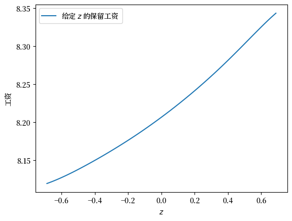
注意保留工资随当前状态 \(z\) 单调递增。
这是因为更高的状态导致个体预测更高的未来工资,增加了等待的价值。
让我们尝试改变失业补偿金并观察其对保留工资的影响:
c_vals = 1, 2, 3

fig, ax = plt.subplots()

for c in c_vals:
    js = JobSearch(c=c)
    f_star = compute_fixed_point(js, verbose=False)
    res_wage_function = np.exp(f_star * (1 - js.β))
    ax.plot(js.z_grid, res_wage_function, label=rf"$c = {c}$ 时的 $\bar w$")

ax.set(xlabel="$z$", ylabel="工资")
ax.legend()
plt.show()
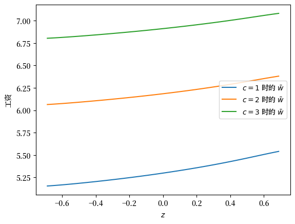
正如预期的那样,更高的失业补偿金在所有状态下都提高了保留工资。
45.4. 失业持续时间#
接下来我们研究平均失业持续时间如何随失业补偿金变化。
为简单起见,我们将初始状态固定在 \(z_t = 0\)。
def compute_unemployment_duration(js, seed=1234):

    f_star = compute_fixed_point(js, verbose=False)
    μ, s, d, ρ, σ, β, c = js.parameters()
    z_grid = js.z_grid
    np.random.seed(seed)

    @jit
    def f_star_function(z):
        return np.interp(z, z_grid, f_star)

    @jit
    def draw_tau(t_max=10_000):
        z = 0
        t = 0

        unemployed = True
        while unemployed and t < t_max:
            # 生成当前工资
            y = np.exp(μ + s * np.random.randn())
            w = np.exp(z) + y
            res_wage = np.exp(f_star_function(z) * (1 - β))
            # 如果最优选择是停止,记录t
            if w >= res_wage:
                unemployed = False
                τ = t
            # 否则增加数据和状态
            else:
                z = ρ * z + d + σ * np.random.randn()
                t += 1
        return τ

    @jit(parallel=True)
    def compute_expected_tau(num_reps=100_000):
        sum_value = 0
        for i in prange(num_reps):
            sum_value += draw_tau()
        return sum_value / num_reps

    return compute_expected_tau()
让我们用一些可能的失业补偿金值来计算失业持续时间:
c_vals = np.linspace(1.0, 10.0, 8)
durations = np.empty_like(c_vals)
for i, c in enumerate(c_vals):
    js = JobSearch(c=c)
    τ = compute_unemployment_duration(js)
    durations[i] = τ
这是可视化结果:
fig, ax = plt.subplots()
ax.plot(c_vals, durations)
ax.set_xlabel("失业补偿金")
ax.set_ylabel("平均失业持续时间")
plt.show()
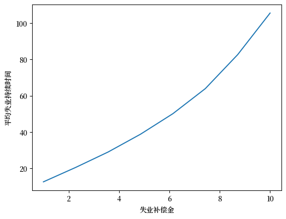
不出所料,当失业补偿金更高时,失业持续时间增加。
这是因为等待的价值随失业补偿金增加。
45.5. 练习#
练习 45.1
研究平均失业持续时间如何随折现因子 \(\beta\) 变化。
你的预期是什么?
结果是否符合你的预期?
解答 练习 45.1
这是一个解决方案
beta_vals = np.linspace(0.94, 0.99, 8)
durations = np.empty_like(beta_vals)
for i, β in enumerate(beta_vals):
    js = JobSearch(β=β)
    τ = compute_unemployment_duration(js)
    durations[i] = τ
fig, ax = plt.subplots()
ax.plot(beta_vals, durations)
ax.set_xlabel(r"$\beta$")
ax.set_ylabel("平均失业持续时间")
plt.show()
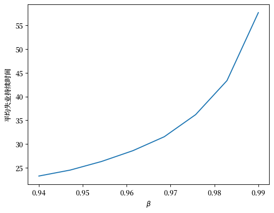
该图显示,更有耐心的个人倾向于等待更长时间才接受报价。