79. 用Pandas处理面板数据#
79.1. 概述#
在之前关于pandas的讲座中,我们学习了如何处理简单的数据集。
计量经济学家经常需要处理更复杂的数据集,比如面板数据。
常见的任务包括:
导入数据、清理数据以及在多个轴上重塑数据。
从面板数据中提取时间序列数据或横截面数据。
对数据进行分组和汇总。
pandas(源自’panel’和’data’这两个词)包含强大且易用的工具,专门用于解决这类问题。
在接下来的内容中,我们将使用来自OECD的实际最低工资面板数据集来创建:
数据在多个维度上的汇总统计
数据集中各国平均最低工资的时间序列
按大洲划分的工资核密度估计
首先,我们将从CSV文件中读取长格式面板数据,并使用pivot_table重塑生成的DataFrame来构建MultiIndex。
使用pandas的merge函数将为我们的DataFrame添加额外的详细信息,并使用groupby函数对数据进行汇总。
79.2. 切片和重塑数据#
我们将读取来自OECD的32个国家的实际最低工资数据集,并将其赋值给realwage。
数据集可通过以下链接访问:
url1 = 'https://raw.githubusercontent.com/QuantEcon/lecture-python/master/source/_static/lecture_specific/pandas_panel/realwage.csv'
import pandas as pd

# 为便于查看,显示数据集前6列
pd.set_option('display.max_columns', 6)

# 将小数点位数减少到2位
pd.options.display.float_format = '{:,.2f}'.format

realwage = pd.read_csv(url1)
让我们看看我们有什么可以使用的数据
realwage.head() # 显示前5行
| Unnamed: 0 | Time | Country | Series | Pay period | value | |
|---|---|---|---|---|---|---|
| 0 | 0 | 2006-01-01 | Ireland | In 2015 constant prices at 2015 USD PPPs | Annual | 17,132.44 |
| 1 | 1 | 2007-01-01 | Ireland | In 2015 constant prices at 2015 USD PPPs | Annual | 18,100.92 |
| 2 | 2 | 2008-01-01 | Ireland | In 2015 constant prices at 2015 USD PPPs | Annual | 17,747.41 |
| 3 | 3 | 2009-01-01 | Ireland | In 2015 constant prices at 2015 USD PPPs | Annual | 18,580.14 |
| 4 | 4 | 2010-01-01 | Ireland | In 2015 constant prices at 2015 USD PPPs | Annual | 18,755.83 |
数据目前是长格式的,当数据有多个维度时,使用这种格式难以进行分析。
我们将使用pivot_table来创建宽格式面板,并使用MultiIndex来处理高维数据。
pivot_table的参数需要指定数据值(values)、索引和在结果数据框中我们所需的列名。
通过在columns参数中传入一个列表,我们可以在列轴上创建一个MultiIndex
realwage = realwage.pivot_table(values='value',
                                index='Time',
                                columns=['Country', 'Series', 'Pay period'])
realwage.head()
| Country | Australia | ... | United States | ||||
|---|---|---|---|---|---|---|---|
| Series | In 2015 constant prices at 2015 USD PPPs | In 2015 constant prices at 2015 USD exchange rates | ... | In 2015 constant prices at 2015 USD PPPs | In 2015 constant prices at 2015 USD exchange rates | ||
| Pay period | Annual | Hourly | Annual | ... | Hourly | Annual | Hourly |
| Time | |||||||
| 2006-01-01 | 20,410.65 | 10.33 | 23,826.64 | ... | 6.05 | 12,594.40 | 6.05 |
| 2007-01-01 | 21,087.57 | 10.67 | 24,616.84 | ... | 6.24 | 12,974.40 | 6.24 |
| 2008-01-01 | 20,718.24 | 10.48 | 24,185.70 | ... | 6.78 | 14,097.56 | 6.78 |
| 2009-01-01 | 20,984.77 | 10.62 | 24,496.84 | ... | 7.58 | 15,756.42 | 7.58 |
| 2010-01-01 | 20,879.33 | 10.57 | 24,373.76 | ... | 7.88 | 16,391.31 | 7.88 |
5 rows × 128 columns
为了更容易地筛选我们的时间序列数据,接下来我们将把索引转换为DateTimeIndex
realwage.index = pd.to_datetime(realwage.index)
type(realwage.index)
pandas.core.indexes.datetimes.DatetimeIndex
该数据框的列包含多层级索引,被称为MultiIndex,各层级按层次结构排序(Country > Series > Pay period)。
MultiIndex是在pandas中管理面板数据最简单且最灵活的方式。
type(realwage.columns)
pandas.core.indexes.multi.MultiIndex
realwage.columns.names
FrozenList(['Country', 'Series', 'Pay period'])
和之前一样,我们可以选择国家(MultiIndex中的最高层级)
realwage['United States'].head()
| Series | In 2015 constant prices at 2015 USD PPPs | In 2015 constant prices at 2015 USD exchange rates | ||
|---|---|---|---|---|
| Pay period | Annual | Hourly | Annual | Hourly |
| Time | ||||
| 2006-01-01 | 12,594.40 | 6.05 | 12,594.40 | 6.05 |
| 2007-01-01 | 12,974.40 | 6.24 | 12,974.40 | 6.24 |
| 2008-01-01 | 14,097.56 | 6.78 | 14,097.56 | 6.78 |
| 2009-01-01 | 15,756.42 | 7.58 | 15,756.42 | 7.58 |
| 2010-01-01 | 16,391.31 | 7.88 | 16,391.31 | 7.88 |
在本讲中,我们将经常使用MultiIndex的堆叠和取消堆叠来将数据框重塑成所需的格式。
.stack()将列MultiIndex的最低层级旋转到行索引(.unstack()执行反向操作 - 你可以试试看)
realwage.stack().head()
/tmp/ipykernel_11348/743219372.py:1: FutureWarning: The previous implementation of stack is deprecated and will be removed in a future version of pandas. See the What's New notes for pandas 2.1.0 for details. Specify future_stack=True to adopt the new implementation and silence this warning.
  realwage.stack().head()
| Country | Australia | Belgium | ... | United Kingdom | United States | |||
|---|---|---|---|---|---|---|---|---|
| Series | In 2015 constant prices at 2015 USD PPPs | In 2015 constant prices at 2015 USD exchange rates | In 2015 constant prices at 2015 USD PPPs | ... | In 2015 constant prices at 2015 USD exchange rates | In 2015 constant prices at 2015 USD PPPs | In 2015 constant prices at 2015 USD exchange rates | |
| Time | Pay period | |||||||
| 2006-01-01 | Annual | 20,410.65 | 23,826.64 | 21,042.28 | ... | 20,376.32 | 12,594.40 | 12,594.40 |
| Hourly | 10.33 | 12.06 | 10.09 | ... | 9.81 | 6.05 | 6.05 | |
| 2007-01-01 | Annual | 21,087.57 | 24,616.84 | 21,310.05 | ... | 20,954.13 | 12,974.40 | 12,974.40 |
| Hourly | 10.67 | 12.46 | 10.22 | ... | 10.07 | 6.24 | 6.24 | |
| 2008-01-01 | Annual | 20,718.24 | 24,185.70 | 21,416.96 | ... | 20,902.87 | 14,097.56 | 14,097.56 |
5 rows × 64 columns
我们也可以传入一个参数来选择我们想要堆叠的层级
realwage.stack(level='Country').head()
/tmp/ipykernel_11348/1205496966.py:1: FutureWarning: The previous implementation of stack is deprecated and will be removed in a future version of pandas. See the What's New notes for pandas 2.1.0 for details. Specify future_stack=True to adopt the new implementation and silence this warning.
  realwage.stack(level='Country').head()
| Series | In 2015 constant prices at 2015 USD PPPs | In 2015 constant prices at 2015 USD exchange rates | |||
|---|---|---|---|---|---|
| Pay period | Annual | Hourly | Annual | Hourly | |
| Time | Country | ||||
| 2006-01-01 | Australia | 20,410.65 | 10.33 | 23,826.64 | 12.06 |
| Belgium | 21,042.28 | 10.09 | 20,228.74 | 9.70 | |
| Brazil | 3,310.51 | 1.41 | 2,032.87 | 0.87 | |
| Canada | 13,649.69 | 6.56 | 14,335.12 | 6.89 | |
| Chile | 5,201.65 | 2.22 | 3,333.76 | 1.42 | |
使用DatetimeIndex可以轻松选择特定的时间段。
选择一年并堆叠MultiIndex的两个较低层级,可以创建我们面板数据的横截面。
realwage.loc['2015'].stack(level=(1, 2)).transpose().head()
/tmp/ipykernel_11348/1065142626.py:1: FutureWarning: The previous implementation of stack is deprecated and will be removed in a future version of pandas. See the What's New notes for pandas 2.1.0 for details. Specify future_stack=True to adopt the new implementation and silence this warning.
  realwage.loc['2015'].stack(level=(1, 2)).transpose().head()
| Time | 2015-01-01 | |||
|---|---|---|---|---|
| Series | In 2015 constant prices at 2015 USD PPPs | In 2015 constant prices at 2015 USD exchange rates | ||
| Pay period | Annual | Hourly | Annual | Hourly |
| Country | ||||
| Australia | 21,715.53 | 10.99 | 25,349.90 | 12.83 |
| Belgium | 21,588.12 | 10.35 | 20,753.48 | 9.95 |
| Brazil | 4,628.63 | 2.00 | 2,842.28 | 1.21 |
| Canada | 16,536.83 | 7.95 | 17,367.24 | 8.35 |
| Chile | 6,633.56 | 2.80 | 4,251.49 | 1.81 |
在本讲后续内容中,我们将使用按国家和时间维度统计的每小时实际最低工资数据框(计量单位为2015年不变价美元)。
为了创建筛选后的数据框(realwage_f),我们可以使用xs方法:在保持更高层级索引(本例中为国家)的同时,选择多级索引中较低层级的值。
realwage_f = realwage.xs(('Hourly', 'In 2015 constant prices at 2015 USD exchange rates'),
                         level=('Pay period', 'Series'), axis=1)
realwage_f.head()
| Country | Australia | Belgium | Brazil | ... | Turkey | United Kingdom | United States |
|---|---|---|---|---|---|---|---|
| Time | |||||||
| 2006-01-01 | 12.06 | 9.70 | 0.87 | ... | 2.27 | 9.81 | 6.05 |
| 2007-01-01 | 12.46 | 9.82 | 0.92 | ... | 2.26 | 10.07 | 6.24 |
| 2008-01-01 | 12.24 | 9.87 | 0.96 | ... | 2.22 | 10.04 | 6.78 |
| 2009-01-01 | 12.40 | 10.21 | 1.03 | ... | 2.28 | 10.15 | 7.58 |
| 2010-01-01 | 12.34 | 10.05 | 1.08 | ... | 2.30 | 9.96 | 7.88 |
5 rows × 32 columns
79.3. 合并数据框和填充空值(NaN 值)#
与SQL等关系型数据库类似,pandas内置了合并数据集的方法。
使用来自WorldData.info的国家信息,我们将使用merge函数将每个国家所属的大洲添加到realwage_f中。
可以通过以下链接访问数据集:
url2 = 'https://raw.githubusercontent.com/QuantEcon/lecture-python/master/source/_static/lecture_specific/pandas_panel/countries.csv'
worlddata = pd.read_csv(url2, sep=';')
worlddata.head()
| Country (en) | Country (de) | Country (local) | ... | Deathrate | Life expectancy | Url | |
|---|---|---|---|---|---|---|---|
| 0 | Afghanistan | Afghanistan | Afganistan/Afqanestan | ... | 13.70 | 51.30 | https://www.laenderdaten.info/Asien/Afghanista... |
| 1 | Egypt | Ägypten | Misr | ... | 4.70 | 72.70 | https://www.laenderdaten.info/Afrika/Aegypten/... |
| 2 | Åland Islands | Ålandinseln | Åland | ... | 0.00 | 0.00 | https://www.laenderdaten.info/Europa/Aland/ind... |
| 3 | Albania | Albanien | Shqipëria | ... | 6.70 | 78.30 | https://www.laenderdaten.info/Europa/Albanien/... |
| 4 | Algeria | Algerien | Al-Jaza’ir/Algérie | ... | 4.30 | 76.80 | https://www.laenderdaten.info/Afrika/Algerien/... |
5 rows × 17 columns
首先,我们将从worlddata中只选择国家和大洲变量,并将列名重命名为Country
worlddata = worlddata[['Country (en)', 'Continent']]
worlddata = worlddata.rename(columns={'Country (en)': 'Country'})
worlddata.head()
| Country | Continent | |
|---|---|---|
| 0 | Afghanistan | Asia |
| 1 | Egypt | Africa |
| 2 | Åland Islands | Europe |
| 3 | Albania | Europe |
| 4 | Algeria | Africa |
我们想要将新的数据框worlddata与realwage_f合并。
pandas的merge函数可以通过行将数据框连接在一起。
我们的数据框将使用国家名称进行合并,这需要我们使用数据框realwage_f的转置,以便两个数据框中的行都对应于国家名称。
realwage_f.transpose().head()
| Time | 2006-01-01 | 2007-01-01 | 2008-01-01 | ... | 2014-01-01 | 2015-01-01 | 2016-01-01 |
|---|---|---|---|---|---|---|---|
| Country | |||||||
| Australia | 12.06 | 12.46 | 12.24 | ... | 12.67 | 12.83 | 12.98 |
| Belgium | 9.70 | 9.82 | 9.87 | ... | 10.01 | 9.95 | 9.76 |
| Brazil | 0.87 | 0.92 | 0.96 | ... | 1.21 | 1.21 | 1.24 |
| Canada | 6.89 | 6.96 | 7.24 | ... | 8.22 | 8.35 | 8.48 |
| Chile | 1.42 | 1.45 | 1.44 | ... | 1.76 | 1.81 | 1.91 |
5 rows × 11 columns
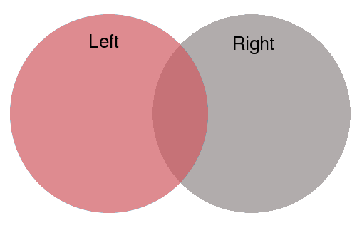
我们可以使用左连接(left)、右连接(right)、内连接(inner)或外连接(outer)来合并我们的数据集:
左连接(left)只包含左侧数据集中的国家
右连接(right)只包含右侧数据集中的国家
内连接(inner)只包含左右数据集共有的国家
外连接(outer)包含左侧和右侧数据集中的任一国家
默认情况下,merge将使用内连接(inner)。
在这个案例中,我们将传入how='left'以保留realwage_f中的所有国家,但丢弃worlddata中不能和realwage_f相匹配的国家。
这在下图中用红色阴影部分表示
我们还需要指定每个数据框中国家名称的位置,这将作为合并数据框的”键(key)”。
我们的”左”(left)数据框(realwage_f.transpose())在索引中包含国家,所以我们设置left_index=True。
我们的”右”(right)数据框(worlddata)在’Country’列中包含国家名称,所以我们设置right_on='Country'
merged = pd.merge(realwage_f.transpose(), worlddata,
                  how='left', left_index=True, right_on='Country')
merged.head()
| 2006-01-01 00:00:00 | 2007-01-01 00:00:00 | 2008-01-01 00:00:00 | ... | 2016-01-01 00:00:00 | Country | Continent | |
|---|---|---|---|---|---|---|---|
| 17.00 | 12.06 | 12.46 | 12.24 | ... | 12.98 | Australia | Australia |
| 23.00 | 9.70 | 9.82 | 9.87 | ... | 9.76 | Belgium | Europe |
| 32.00 | 0.87 | 0.92 | 0.96 | ... | 1.24 | Brazil | South America |
| 100.00 | 6.89 | 6.96 | 7.24 | ... | 8.48 | Canada | North America |
| 38.00 | 1.42 | 1.45 | 1.44 | ... | 1.91 | Chile | South America |
5 rows × 13 columns
在 realwage_f 中出现但在 worlddata 中未出现的国家,其 Continent 列将显示 NaN。
要检查是否发生这种情况,我们可以在 Continent 列上使用 .isnull() 并过滤合并后的数据框
merged[merged['Continent'].isnull()]
| 2006-01-01 00:00:00 | 2007-01-01 00:00:00 | 2008-01-01 00:00:00 | ... | 2016-01-01 00:00:00 | Country | Continent | |
|---|---|---|---|---|---|---|---|
| NaN | 3.42 | 3.74 | 3.87 | ... | 5.28 | Korea | NaN |
| NaN | 0.23 | 0.45 | 0.39 | ... | 0.55 | Russian Federation | NaN |
| NaN | 1.50 | 1.64 | 1.71 | ... | 2.08 | Slovak Republic | NaN |
3 rows × 13 columns
我们有三个缺失值!
处理 NaN 值的一个方式是创建一个包含这些国家及其对应大洲的字典。
.map() 将会把 merged['Country'] 中的国家与字典中的大洲进行匹配。
注意那些不在我们字典中的国家是如何被映射为 NaN 的
missing_continents = {'Korea': 'Asia',
                      'Russian Federation': 'Europe',
                      'Slovak Republic': 'Europe'}

merged['Country'].map(missing_continents)
17.00        NaN
23.00        NaN
32.00        NaN
100.00       NaN
38.00        NaN
108.00       NaN
41.00        NaN
225.00       NaN
53.00        NaN
58.00        NaN
45.00        NaN
68.00        NaN
233.00       NaN
86.00        NaN
88.00        NaN
91.00        NaN
NaN         Asia
117.00       NaN
122.00       NaN
123.00       NaN
138.00       NaN
153.00       NaN
151.00       NaN
174.00       NaN
175.00       NaN
NaN       Europe
NaN       Europe
198.00       NaN
200.00       NaN
227.00       NaN
241.00       NaN
240.00       NaN
Name: Country, dtype: object
我们不想用这个映射覆盖整个序列。
.fillna() 只会用映射值填充 merged['Continent'] 中的 NaN 值,同时保持列中的其他值不变
merged['Continent'] = merged['Continent'].fillna(merged['Country'].map(missing_continents))

# 检查大洲是否被正确映射
merged[merged['Country'] == 'Korea']
| 2006-01-01 00:00:00 | 2007-01-01 00:00:00 | 2008-01-01 00:00:00 | ... | 2016-01-01 00:00:00 | Country | Continent | |
|---|---|---|---|---|---|---|---|
| NaN | 3.42 | 3.74 | 3.87 | ... | 5.28 | Korea | Asia |
1 rows × 13 columns
我们把美洲合并成一个大洲 – 这样可以让我们后面的可视化效果更好。
为此,我们将使用.replace()并遍历一个包含我们想要替换的大洲的值的列表
replace = ['Central America', 'North America', 'South America']

for country in replace:
    merged['Continent'] = merged['Continent'].replace(
                                {country:'America'})
现在我们已经将所有想要的数据都放在一个DataFrame中,我们将把它重新整形成带有MultiIndex的面板形式。
我们还应该使用.sort_index()来确保对索引进行排序,这样我们之后可以高效地筛选数据框。
默认情况下,层级将按照从上到下的顺序排序
merged = merged.set_index(['Continent', 'Country']).sort_index()
merged.head()
| 2006-01-01 | 2007-01-01 | 2008-01-01 | ... | 2014-01-01 | 2015-01-01 | 2016-01-01 | ||
|---|---|---|---|---|---|---|---|---|
| Continent | Country | |||||||
| America | Brazil | 0.87 | 0.92 | 0.96 | ... | 1.21 | 1.21 | 1.24 |
| Canada | 6.89 | 6.96 | 7.24 | ... | 8.22 | 8.35 | 8.48 | |
| Chile | 1.42 | 1.45 | 1.44 | ... | 1.76 | 1.81 | 1.91 | |
| Colombia | 1.01 | 1.02 | 1.01 | ... | 1.13 | 1.13 | 1.12 | |
| Costa Rica | NaN | NaN | NaN | ... | 2.41 | 2.56 | 2.63 |
5 rows × 11 columns
在合并过程中,我们丢失了DatetimeIndex,因为我们合并的列不是日期时间格式的
merged.columns
Index([2006-01-01 00:00:00, 2007-01-01 00:00:00, 2008-01-01 00:00:00,
       2009-01-01 00:00:00, 2010-01-01 00:00:00, 2011-01-01 00:00:00,
       2012-01-01 00:00:00, 2013-01-01 00:00:00, 2014-01-01 00:00:00,
       2015-01-01 00:00:00, 2016-01-01 00:00:00],
      dtype='object')
现在我们已经将合并的列设置为索引,我们可以使用.to_datetime()重新创建一个DatetimeIndex
merged.columns = pd.to_datetime(merged.columns)
merged.columns = merged.columns.rename('Time')
merged.columns
DatetimeIndex(['2006-01-01', '2007-01-01', '2008-01-01', '2009-01-01',
               '2010-01-01', '2011-01-01', '2012-01-01', '2013-01-01',
               '2014-01-01', '2015-01-01', '2016-01-01'],
              dtype='datetime64[ns]', name='Time', freq=None)
一般来说DatetimeIndex在行轴上运作起来更加顺畅,所以我们将对merged进行转置
merged = merged.transpose()
merged.head()
| Continent | America | ... | Europe | ||||
|---|---|---|---|---|---|---|---|
| Country | Brazil | Canada | Chile | ... | Slovenia | Spain | United Kingdom |
| Time | |||||||
| 2006-01-01 | 0.87 | 6.89 | 1.42 | ... | 3.92 | 3.99 | 9.81 |
| 2007-01-01 | 0.92 | 6.96 | 1.45 | ... | 3.88 | 4.10 | 10.07 |
| 2008-01-01 | 0.96 | 7.24 | 1.44 | ... | 3.96 | 4.14 | 10.04 |
| 2009-01-01 | 1.03 | 7.67 | 1.52 | ... | 4.08 | 4.32 | 10.15 |
| 2010-01-01 | 1.08 | 7.94 | 1.56 | ... | 4.81 | 4.30 | 9.96 |
5 rows × 32 columns
79.4. 数据分组和汇总#
对于理解大型面板数据集来说,数据分组和汇总特别有用。
一种简单的数据汇总方法是在数据框上调用聚合方法,比如.mean()或.max()。
例如,我们可以计算2006年至2016年期间每个国家的平均实际最低工资(默认是按行聚合)
merged.mean().head(10)
Continent  Country
America    Brazil          1.09
           Canada          7.82
           Chile           1.62
           Colombia        1.07
           Costa Rica      2.53
           Mexico          0.53
           United States   7.15
Asia       Israel          5.95
           Japan           6.18
           Korea           4.22
dtype: float64
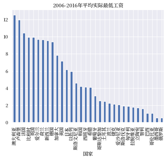
使用这个数据序列,我们可以绘制数据集中每个国家过去十年的平均实际最低工资
import matplotlib.pyplot as plt
import matplotlib as mpl
FONTPATH = "fonts/SourceHanSerifSC-SemiBold.otf"
mpl.font_manager.fontManager.addfont(FONTPATH)
plt.rcParams['font.family'] = ['Source Han Serif SC']

import seaborn as sns
sns.set_theme()
sns.set(font='Source Han Serif SC')

# 导入中文国家名称
map_url='https://raw.githubusercontent.com/QuantEcon/lecture-python.zh-cn/refs/heads/main/lectures/_static/country_map.csv'
country_map = pd.read_csv(map_url).set_index('English')['Chinese']
merged.T.groupby(level='Continent').mean()
| Time | 2006-01-01 | 2007-01-01 | 2008-01-01 | ... | 2014-01-01 | 2015-01-01 | 2016-01-01 |
|---|---|---|---|---|---|---|---|
| Continent | |||||||
| America | 2.80 | 2.85 | 2.99 | ... | 3.22 | 3.26 | 3.30 |
| Asia | 4.29 | 4.44 | 4.45 | ... | 4.86 | 5.10 | 5.44 |
| Australia | 10.25 | 10.73 | 10.76 | ... | 11.25 | 11.52 | 11.73 |
| Europe | 4.80 | 4.94 | 4.99 | ... | 5.17 | 5.48 | 5.57 |
4 rows × 11 columns
merged.mean().sort_values(ascending=False).plot(
          kind='bar',
          title="2006-2016年平均实际最低工资")

# 设置国家标签
country_labels = merged.mean().sort_values(
    ascending=False).index.get_level_values('Country').tolist()

# 将国家名称从英文转换为中文
country_labels_cn = [country_map[label] for label
                     in country_labels]
plt.xticks(range(0, len(country_labels)), country_labels_cn)
plt.xlabel('国家')

plt.show()
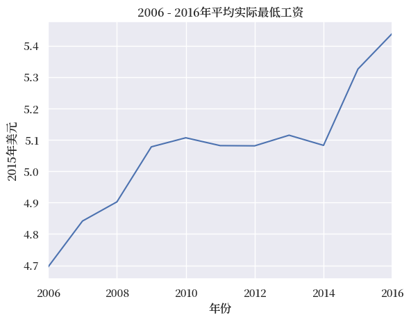
通过向.mean()传入axis=1参数可以对列进行聚合(得到所有国家随时间变化的平均最低工资)
merged.mean(axis=1).head()
Time
2006-01-01   4.69
2007-01-01   4.84
2008-01-01   4.90
2009-01-01   5.08
2010-01-01   5.11
dtype: float64
我们可以将这个时间序列绘制成折线图
merged.mean(axis=1).plot()
plt.title('2006 - 2016年平均实际最低工资')
plt.ylabel('2015年美元')
plt.xlabel('年份')
plt.show()
我们也可以指定MultiIndex的一个层级(在列轴上)来进行聚合
merged.T.groupby(level='Continent').mean().head()
| Time | 2006-01-01 | 2007-01-01 | 2008-01-01 | ... | 2014-01-01 | 2015-01-01 | 2016-01-01 |
|---|---|---|---|---|---|---|---|
| Continent | |||||||
| America | 2.80 | 2.85 | 2.99 | ... | 3.22 | 3.26 | 3.30 |
| Asia | 4.29 | 4.44 | 4.45 | ... | 4.86 | 5.10 | 5.44 |
| Australia | 10.25 | 10.73 | 10.76 | ... | 11.25 | 11.52 | 11.73 |
| Europe | 4.80 | 4.94 | 4.99 | ... | 5.17 | 5.48 | 5.57 |
4 rows × 11 columns
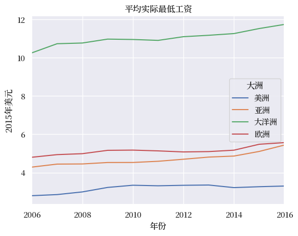
我们可以将每个大洲的平均最低工资绘制成时间序列图
continent_map = {'Asia':'亚洲',
                 'Europe':'欧洲',
                 'America':'美洲',
                 'Australia':'大洋洲'}

(merged.T
       .groupby(level='Continent')
       .mean()
       .T.rename(columns=continent_map)
).plot()
plt.title('平均实际最低工资')
plt.ylabel('2015年美元')
plt.xlabel('年份')
plt.legend(title='大洲')
plt.show()
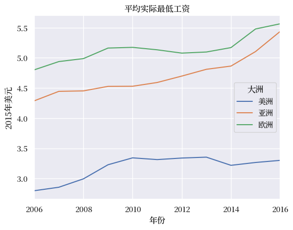
出于绘图目的,我们将去掉澳大利亚这个大洲
merged = merged.drop('Australia', level='Continent', axis=1)
(merged.T
      .groupby(level='Continent')
      .mean().T
      .rename(columns=continent_map)
      ).plot()
plt.title('平均实际最低工资')
plt.legend(title='大洲')
plt.ylabel('2015年美元')
plt.xlabel('年份')
plt.show()
.describe() 可以快速获取一些常见的描述性统计量的汇总结果
merged.stack().describe()
/tmp/ipykernel_11348/4288984536.py:1: FutureWarning: The previous implementation of stack is deprecated and will be removed in a future version of pandas. See the What's New notes for pandas 2.1.0 for details. Specify future_stack=True to adopt the new implementation and silence this warning.
  merged.stack().describe()
| Continent | America | Asia | Europe |
|---|---|---|---|
| count | 69.00 | 44.00 | 200.00 |
| mean | 3.19 | 4.70 | 5.15 |
| std | 3.02 | 1.56 | 3.82 |
| min | 0.52 | 2.22 | 0.23 |
| 25% | 1.03 | 3.37 | 2.02 |
| 50% | 1.44 | 5.48 | 3.54 |
| 75% | 6.96 | 5.95 | 9.70 |
| max | 8.48 | 6.65 | 12.39 |
让我们更深入地了解 groupby 的工作原理。
groupby 操作遵循一个称为”拆分-应用-合并”的模式:
首先,数据会按照指定的一个或多个键被拆分成多个组
然后,对每个组分别执行相同的操作或计算
最后,将所有组的结果合并成一个新的数据结构
这种模式使我们能够对数据子集进行灵活的分组分析。
groupby 方法实现了这个过程的第一步,创建一个新的 DataFrameGroupBy 对象,将数据拆分成组。
让我们再次按大洲拆分 merged,这次使用 groupby 函数,并将生成的对象命名为 grouped
grouped = merged.T.groupby(level='Continent')
grouped.keys
在对象上调用groupby方法时,该函数会被应用于每个组,运算结果会被合并到一个新的数据结构中。
例如,我们可以使用.size()返回数据集中每个大洲的国家数量。
在这种情况下,我们的新数据结构是一个Series
grouped.size()
Continent
America     7
Asia        4
Europe     19
dtype: int64
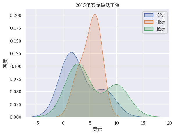
通过调用 .get_group() 来返回单个组中的国家,我们可以为每个大洲创建2016年实际最低工资分布的核密度估计。
grouped.groups.keys() 将返回 groupby 对象中的键
continents = grouped.groups.keys()

for continent in continents:
    sns.kdeplot(grouped.get_group(continent).T.loc['2015'].unstack(),
                label=continent_map[continent], fill=True)

plt.title('2015年实际最低工资')
plt.xlabel('美元')
plt.ylabel('密度')
plt.legend()
plt.show()
79.5. 总结#
本讲座介绍了pandas的一些高级特性,包括多级索引、合并、分组和绘图。
在面板数据分析中,其他可能有用的工具包括xarray,这是一个将pandas扩展到N维数据结构的Python包。
79.6. 练习#
练习 79.1
在这些练习中,你将使用来自Eurostat的按年龄和性别划分的欧洲就业率数据集。
可以通过以下链接访问数据集:
url3 = 'https://raw.githubusercontent.com/QuantEcon/lecture-python/master/source/_static/lecture_specific/pandas_panel/employ.csv'
读取 CSV 文件会返回一个长格式的面板数据集。使用 .pivot_table() 构建一个带有 MultiIndex 列的宽格式数据框。
首先探究数据框和 MultiIndex 层级中可用的变量。
编写一个程序,快速返回 MultiIndex 中的所有值。
解答 练习 79.1
employ = pd.read_csv(url3)
employ = employ.pivot_table(values='Value',
                            index=['DATE'],
                            columns=['UNIT','AGE', 'SEX', 'INDIC_EM', 'GEO'])
employ.index = pd.to_datetime(employ.index) # 确保日期为 datetime 格式
employ.head()
| UNIT | Percentage of total population | ... | Thousand persons | ||||
|---|---|---|---|---|---|---|---|
| AGE | From 15 to 24 years | ... | From 55 to 64 years | ||||
| SEX | Females | ... | Total | ||||
| INDIC_EM | Active population | ... | Total employment (resident population concept - LFS) | ||||
| GEO | Austria | Belgium | Bulgaria | ... | Switzerland | Turkey | United Kingdom |
| DATE | |||||||
| 2007-01-01 | 56.00 | 31.60 | 26.00 | ... | NaN | 1,282.00 | 4,131.00 |
| 2008-01-01 | 56.20 | 30.80 | 26.10 | ... | NaN | 1,354.00 | 4,204.00 |
| 2009-01-01 | 56.20 | 29.90 | 24.80 | ... | NaN | 1,449.00 | 4,193.00 |
| 2010-01-01 | 54.00 | 29.80 | 26.60 | ... | 640.00 | 1,583.00 | 4,186.00 |
| 2011-01-01 | 54.80 | 29.80 | 24.80 | ... | 661.00 | 1,760.00 | 4,164.00 |
5 rows × 1440 columns
由于这是一个大型数据集,因此探索可用的层级和变量很有用
employ.columns.names
FrozenList(['UNIT', 'AGE', 'SEX', 'INDIC_EM', 'GEO'])
可以通过循环快速获取层级中的变量
for name in employ.columns.names:
    print(name, employ.columns.get_level_values(name).unique())
UNIT Index(['Percentage of total population', 'Thousand persons'], dtype='object', name='UNIT')
AGE Index(['From 15 to 24 years', 'From 25 to 54 years', 'From 55 to 64 years'], dtype='object', name='AGE')
SEX Index(['Females', 'Males', 'Total'], dtype='object', name='SEX')
INDIC_EM Index(['Active population', 'Total employment (resident population concept - LFS)'], dtype='object', name='INDIC_EM')
GEO Index(['Austria', 'Belgium', 'Bulgaria', 'Croatia', 'Cyprus', 'Czech Republic',
       'Denmark', 'Estonia', 'Euro area (17 countries)',
       'Euro area (18 countries)', 'Euro area (19 countries)',
       'European Union (15 countries)', 'European Union (27 countries)',
       'European Union (28 countries)', 'Finland',
       'Former Yugoslav Republic of Macedonia, the', 'France',
       'France (metropolitan)',
       'Germany (until 1990 former territory of the FRG)', 'Greece', 'Hungary',
       'Iceland', 'Ireland', 'Italy', 'Latvia', 'Lithuania', 'Luxembourg',
       'Malta', 'Netherlands', 'Norway', 'Poland', 'Portugal', 'Romania',
       'Slovakia', 'Slovenia', 'Spain', 'Sweden', 'Switzerland', 'Turkey',
       'United Kingdom'],
      dtype='object', name='GEO')
练习 79.2
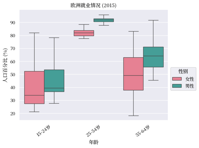
筛选上述数据框,仅保留以’活动人口’百分比表示的就业数据。
使用seaborn绘制一个按年龄和性别分组的2015年就业率箱线图。
提示
GEO包含地区和国家。
解答 练习 79.2
为了更方便地按国家筛选,将GEO调整到最上层并对MultiIndex进行排序
employ.columns = employ.columns.swaplevel(0,-1)
employ = employ.sort_index(axis=1)
我们需要删除GEO中一些不是国家的项。
一个快速去除欧盟地区的方法是使用列表推导式来查找GEO中以’Euro’开头的层级值。
geo_list = employ.columns.get_level_values('GEO').unique().tolist()
countries = [x for x in geo_list if not x.startswith('Euro')]
employ = employ[countries]
employ.columns.get_level_values('GEO').unique()
Index(['Austria', 'Belgium', 'Bulgaria', 'Croatia', 'Cyprus', 'Czech Republic',
       'Denmark', 'Estonia', 'Finland',
       'Former Yugoslav Republic of Macedonia, the', 'France',
       'France (metropolitan)',
       'Germany (until 1990 former territory of the FRG)', 'Greece', 'Hungary',
       'Iceland', 'Ireland', 'Italy', 'Latvia', 'Lithuania', 'Luxembourg',
       'Malta', 'Netherlands', 'Norway', 'Poland', 'Portugal', 'Romania',
       'Slovakia', 'Slovenia', 'Spain', 'Sweden', 'Switzerland', 'Turkey',
       'United Kingdom'],
      dtype='object', name='GEO')
仅选择数据框中活动人口的就业百分比
employ_f = employ.xs(('Percentage of total population', 'Active population'),
                     level=('UNIT', 'INDIC_EM'),
                     axis=1)
employ_f.head()
| GEO | Austria | ... | United Kingdom | ||||
|---|---|---|---|---|---|---|---|
| AGE | From 15 to 24 years | ... | From 55 to 64 years | ||||
| SEX | Females | Males | Total | ... | Females | Males | Total |
| DATE | |||||||
| 2007-01-01 | 56.00 | 62.90 | 59.40 | ... | 49.90 | 68.90 | 59.30 |
| 2008-01-01 | 56.20 | 62.90 | 59.50 | ... | 50.20 | 69.80 | 59.80 |
| 2009-01-01 | 56.20 | 62.90 | 59.50 | ... | 50.60 | 70.30 | 60.30 |
| 2010-01-01 | 54.00 | 62.60 | 58.30 | ... | 51.10 | 69.20 | 60.00 |
| 2011-01-01 | 54.80 | 63.60 | 59.20 | ... | 51.30 | 68.40 | 59.70 |
5 rows × 306 columns
在绘制分组箱形图之前删除”总计”值
employ_f = employ_f.drop('Total', level='SEX', axis=1)
box = employ_f.loc['2015'].unstack().reset_index()
box['SEX'] = box['SEX'].map({'Males': '男性', 'Females': '女性'})
sns.boxplot(x="AGE", y=0, hue="SEX",
            data=box, palette=("husl"),
            showfliers=False)
plt.legend(title='性别',
           bbox_to_anchor=(1, 0.5))

age_labels = {
    'From 15 to 24 years': '15-24岁',
    'From 25 to 54 years': '25-54岁',
    'From 55 to 64 years': '55-64岁',
    'From 65 to 74 years': '65-74岁'
}

xtick_labels = [age_labels.get(label.get_text(),
                label.get_text())
                for label in plt.gca().get_xticklabels()]
xticks = plt.gca().get_xticks()
plt.xticks(ticks=xticks, labels=xtick_labels, rotation=35)
plt.xticks(rotation=35)
plt.xlabel('年龄')
plt.ylabel('人口百分比 (%)')
plt.title('欧洲就业情况 (2015)')
plt.show()