8. 基础概率论与矩阵#
本讲座使用矩阵代数来说明概率论的一些基本概念。
在对基本概念进行简要定义后,我们将使用矩阵和向量来描述概率分布。
我们将学习的概念包括:
联合概率分布
给定联合分布的边缘分布
条件概率分布
两个随机变量的统计独立性
与指定边缘分布相关的联合分布
耦合
Copula函数
两个独立随机变量之和的概率分布
边缘分布的卷积
定义概率分布的参数
作为数据摘要的充分统计量
我们将使用矩阵来表示二元概率分布,使用向量来表示一元概率分布
除了Anaconda中已有的库外,本讲还需要以下库:
!pip install prettytable
和平常一样,我们先导入一些库
import numpy as np
import matplotlib.pyplot as plt
import matplotlib as mpl
FONTPATH = "fonts/SourceHanSerifSC-SemiBold.otf"
mpl.font_manager.fontManager.addfont(FONTPATH)
plt.rcParams['font.family'] = ['Source Han Serif SC']

import prettytable as pt
from mpl_toolkits.mplot3d import Axes3D
from matplotlib_inline.backend_inline import set_matplotlib_formats
set_matplotlib_formats('retina')
8.1. 基本概念概述#
我们将简要定义概率空间、概率测度和随机变量。
在本讲座的大部分内容中,这些概念将不会被反复提及,但它们构成我们所讨论其他主题的基础。
设 \(\Omega\) 为可能的基本结果集,设 \(\omega \in \Omega\) 为一个特定的基本结果。
设 \(\mathcal{G} \subset \Omega\) 为 \(\Omega\) 的一个子集。
设 \(\mathcal{F}\) 为这些子集 \(\mathcal{G} \subset \Omega\) 的集合。
对 \(\Omega,\mathcal{F}\) 这一配对就是我们想要赋予概率测度的概率空间。
概率测度 \(\mu\) 将可能的基本结果集 \(\mathcal{G} \in \mathcal{F}\) 映射到0和1之间的实数
即 \(X\) 属于 \(A\) 的”概率”,记为 \( \textrm{Prob}\{X\in A\}\)。
随机变量 \(X(\omega)\) 是基本结果 \(\omega \in \Omega\) 的一个函数。
随机变量 \(X(\omega)\) 具有由基础概率测度 \(\mu\) 和函数 \(X(\omega)\) 诱导的概率分布:
其中 \({\mathcal G}\) 是 \(\Omega\) 的子集,满足 \(X(\omega) \in A\)。
我们称这为随机变量 \(X\) 的诱导概率分布。
在实际工作中,应用统计学家往往不从底层的概率空间 \(\Omega,\mathcal{F}\) 和概率测度 \(\mu\) 出发进行显式推导,而是直接为某个随机变量给定其诱导分布的函数形式。
本讲以及此后的多篇讲座都将采用这种做法。
8.2. 概率是什么意思?#
在深入讨论之前,我们先简单谈谈概率的含义,以及概率论与统计学的关系。
我们在 quantecon 讲座 https://python.quantecon.org/prob_meaning.html 和 https://python.quantecon.org/navy_captain.html 中也涉及了这些主题。
在本讲座的大部分内容中,我们讨论的都是固定的”总体”概率分布。
这些概率分布是纯粹的数学对象。
要理解统计学家如何将概率与数据联系起来,关键是理解以下概念:
从概率分布中进行单次抽样
从同一概率分布中重复地进行独立同分布(i.i.d.)抽样,得到”样本”或”观测值”
统计量,定义为样本序列的函数
经验分布或直方图(将观测数据分箱后的经验分布),用于记录观察到的相对频率
总体概率分布可以看作是一长串 i.i.d. 抽样试验中相对频率的期望值。以下数学工具定义了何为期望的相对频率:
大数定律(LLN)
中心极限定理(CLT)
标量示例
设\(X\)是一个标量随机变量,它可以取\(I\)个可能的值\(0, 1, 2, \ldots, I-1\),其概率为
其中
我们有时写作
这是一种简写方式,表示随机变量\(X\)由概率分布\( \{{f_i}\}_{i=0}^{I-1}\)描述。
考虑从\(X\)中抽取\(N\)个独立同分布的样本\(x_0, x_1, \dots , x_{N-1}\)。
“独立同分布”(i.i.d.)这个术语中,”同分布”和”独立”各自意味着什么?
“同分布”意味着每次抽样都来自相同的分布。
“独立”意味着联合分布等于边缘分布的乘积,即:
我们定义一个经验分布如下。
对于每个 \(i = 0,\dots,I-1\),令
将概率论与统计学联系起来的关键思想是大数定律和中心极限定理
大数定律:
大数定律(LLN)表明 \(\tilde {f_i} \to f_i \text{ 当 } N \to \infty\)
中心极限定理:
中心极限定理(CLT)描述了 \(\tilde {f_i} \to f_i\) 的收敛速率
备注
对于”频率学派”统计学家来说,预期相对频率就是概率分布的全部含义。
但对贝叶斯学派来说,概率的含义有所不同——在一定程度上是主观且带有个人色彩的。
之所以说”在一定程度上”,是因为贝叶斯学派同样会关注相对频率。
8.3. 表示概率分布#
概率分布 \(\textrm{Prob} (X \in A)\) 可以用其**累积分布函数(CDF)**来描述
有时候(但不总是如此),随机变量也可以用与其累积分布函数相对应的密度函数 \(f(x)\) 来描述:
这里 \(B\) 表示我们要求 \(X\) 落在其中的值的集合。
在概率密度存在的情况下,一个概率分布可以通过其累积分布函数或概率密度函数来表征。
对于离散型随机变量:
\(X\) 的可能值的数量是有限的或可数无限的
我们用概率质量函数(一个非负且和为1的序列)代替密度
在类似 (8.1) 这样的关联累积分布函数和概率质量函数的公式中,我们用求和代替积分
在本讲中,我们主要讨论离散随机变量。
这样做使我们能够基本上把所用工具限定在线性代数范围内。
稍后我们将简要讨论如何用离散型随机变量来近似连续型随机变量。
8.4. 单变量概率分布#
在本讲中,我们将主要讨论离散型随机变量,但也会简单介绍一下连续型随机变量。
8.4.1. 离散随机变量#
设 \(X\) 是一个离散随机变量,其可能取值为:\(i=0,1,\ldots,I-1 = \bar{X}\)。
这里,我们将最大索引设定为 \(I-1\),是因为这与Python的索引约定(从0开始)很好地对应。
定义 \(f_i \equiv \textrm{Prob}\{X=i\}\) 并构造非负向量
其中对每个 \(i\) 都有 \(f_{i} \in [0,1]\) 且 \(\sum_{i=0}^{I-1}f_i=1\)。
这个向量定义了一个概率质量函数。
概率分布 (8.2) 的参数为 \(\{f_{i}\}_{i=0,1, \cdots ,I-2}\),因为 \(f_{I-1} = 1-\sum_{i=0}^{I-2}f_{i}\)。
这些参数确定了分布的形状。
(有时 \(I = \infty\)。)
这种”非参数”分布的”参数”数量与随机变量的可能值数量相同。
我们经常使用由少量参数表征的特殊分布。
在这些特殊的参数分布中,
其中 \(\theta\) 是一个参数向量,其维度远小于 \(I\)。
注意:
统计模型是由一组参数刻画的联合概率分布。
参数的概念与充分统计量的概念密切相关。
统计量是数据集的非线性函数。
充分统计量旨在总结数据集中包含的关于参数的所有信息。
充分统计量始终是相对于某一特定的统计模型而言的。
充分统计量是人工智能用来概括或压缩大数据集的关键工具
R. A. Fisher 提供了信息的严格定义 – 参见 https://baike.baidu.com/item/费希尔信息/22742376
几何分布是参数概率分布的一个例子。
它的描述如下:
显然,\(\sum_{i=0}^{\infty}f_i=1\)。
设\(\theta\)是由\(f\)描述的分布的参数向量,则:
8.4.2. 连续随机变量#
设\(X\)是一个取值为\(X \in \tilde{X}\equiv[X_U,X_L]\)的连续随机变量,其分布具有参数\(\theta\)。
其中\(A\)是\(\tilde{X}\)的一个子集,且:
8.5. 二元概率分布#
现在我们将讨论二元联合分布。
首先,我们将关注两个离散随机变量的情况。
设\(X,Y\)是两个离散随机变量,它们的取值为:
它们的联合分布可以用一个矩阵表示
其中矩阵的元素为
且满足
8.6. 边缘概率分布#
由联合分布可以推出边缘分布:
例如,设\((X,Y)\)的联合分布为
由此得到的边缘分布为:
题外话: 如果两个随机变量 \(X,Y\) 是连续的且具有联合密度 \(f(x,y)\),则边缘分布可以通过以下方式计算:
8.7. 条件概率分布#
条件概率的定义如下:
其中 \(A, B\) 是两个事件。
对于一对离散随机变量,它们的条件分布可以表示为:
其中 \(i=0, \ldots,I-1, \quad j=0,\ldots,J-1\)。
注意:
注: 条件概率的定义实际上蕴含了贝叶斯定理:
对于上述联合分布 (8.3)
8.8. 转移概率矩阵#
8.8 转移概率矩阵
考虑两个随机变量的如下联合概率分布。
设 \(X, Y\) 为离散随机变量,其联合分布为
其中 \(i=0,\ldots,I-1;\; j=0,\ldots,J-1\),并且
相应的条件分布为
我们可以定义一个转移概率矩阵 \(P\),其第 \(i,j\) 个元素为
其中
第一行给出在 \(X=0\) 条件下 \(Y=j\)(\(j=0,1\))的概率;第二行给出在 \(X=1\) 条件下 \(Y=j\)(\(j=0,1\))的概率。
注意:
\(\sum_j \rho_{ij}=\dfrac{\sum_j \rho_{ij}}{\sum_j \rho_{ij}}=1\),因此转移矩阵 \(P\) 的每一行都是一个概率分布(列一般不是)。
8.9. 应用:时间序列的预测#
假设只有两个时期:
\(t=0\) 表示”今天”
\(t=1\) 表示”明天”
令 \(X(0)\) 为在 \(t=0\) 时实现的随机变量,\(X(1)\) 为在 \(t=1\) 时实现的随机变量。
假设
则 \(f_{ij}\) 是 \([X(0), X(1)]\) 的联合分布。其对应的条件分布为
备注:
该公式是应用经济学中进行时间序列预测的常用工具。
8.10. 统计独立性#
如果随机变量 X 和 Y 满足以下条件,则称它们是统计独立的:
其中
条件分布为:
8.11. 均值和方差#
离散随机变量 \(X\) 的均值和方差为:
具有密度\(f_{X}(x)\)的连续随机变量的均值和方差为
让我们用一个小故事来说明这个例子。
假设你去参加一个工作面试,你要么通过要么失败。
你有5%的机会通过面试,而且你知道如果通过的话,你的日薪会在300~400之间均匀分布。
我们可以用以下概率来描述你的日薪这个离散-连续变量:
让我们先生成一个随机样本并计算样本矩。
x = np.random.rand(1_000_000)
# x[x > 0.95] = 100*x[x > 0.95]+300
x[x > 0.95] = 100*np.random.rand(len(x[x > 0.95]))+300
x[x <= 0.95] = 0

μ_hat = np.mean(x)
σ2_hat = np.var(x)

print("样本均值是: ", μ_hat, "\n样本方差是: ", σ2_hat)
样本均值是:  17.521480687448843
样本方差是:  5865.45517436778
可以计算解析均值和方差:
mean = 0.0005*0.5*(400**2 - 300**2)
var = 0.95*17.5**2+0.0005/3*((400-17.5)**3-(300-17.5)**3)
print("mean: ", mean)
print("variance: ", var)
mean:  17.5
variance:  5860.416666666666
8.12. 一些二元分布的矩阵表示#
让我们用矩阵来表示联合分布、条件分布、边缘分布以及二元随机变量的均值和方差。
下表展示了一个二元随机变量的概率分布。
边缘分布为
抽样:
让我们写一段 Python 代码,用来生成大样本并计算相对频率。
这段代码将帮助我们检验”抽样”分布是否与”总体”分布一致——从而确认总体分布确实给出了在大样本中应当期望 的相对频率。
# 指定参数
xs = np.array([0, 1])
ys = np.array([10, 20])
f = np.array([[0.3, 0.2], [0.1, 0.4]])
f_cum = np.cumsum(f)

# 生成随机数
p = np.random.rand(1_000_000)
x = np.vstack([xs[1]*np.ones(p.shape), ys[1]*np.ones(p.shape)])
# 映射到二元分布

x[0, p < f_cum[2]] = xs[1]
x[1, p < f_cum[2]] = ys[0]

x[0, p < f_cum[1]] = xs[0]
x[1, p < f_cum[1]] = ys[1]

x[0, p < f_cum[0]] = xs[0]
x[1, p < f_cum[0]] = ys[0]
print(x)
[[ 0.  1.  0. ...  1.  0.  0.]
 [10. 20. 10. ... 20. 10. 10.]]
在这里,我们使用逆CDF技术来从联合分布\(F\)中生成样本。
# 边缘分布
xp = np.sum(x[0, :] == xs[0])/1_000_000
yp = np.sum(x[1, :] == ys[0])/1_000_000

# 打印输出
print("x的边缘分布")
xmtb = pt.PrettyTable()
xmtb.field_names = ['x值', 'x概率']
xmtb.add_row([xs[0], xp])
xmtb.add_row([xs[1], 1-xp])
print(xmtb)

print("\ny的边缘分布")
ymtb = pt.PrettyTable()
ymtb.field_names = ['y值', 'y概率']
ymtb.add_row([ys[0], yp])
ymtb.add_row([ys[1], 1-yp])
print(ymtb)
x的边缘分布
+-----+---------------------+
| x值 |        x概率        |
+-----+---------------------+
|  0  |       0.500597      |
|  1  | 0.49940300000000004 |
+-----+---------------------+

y的边缘分布
+-----+--------------------+
| y值 |       y概率        |
+-----+--------------------+
|  10 |      0.400105      |
|  20 | 0.5998950000000001 |
+-----+--------------------+
# 条件分布
xc1 = x[0, x[1, :] == ys[0]]
xc2 = x[0, x[1, :] == ys[1]]
yc1 = x[1, x[0, :] == xs[0]]
yc2 = x[1, x[0, :] == xs[1]]

xc1p = np.sum(xc1 == xs[0])/len(xc1)
xc2p = np.sum(xc2 == xs[0])/len(xc2)
yc1p = np.sum(yc1 == ys[0])/len(yc1)
yc2p = np.sum(yc2 == ys[0])/len(yc2)

# 打印输出
print("x的条件分布")
xctb = pt.PrettyTable()
xctb.field_names = ['y值', 'x=0的概率', 'x=1的概率']
xctb.add_row([ys[0], xc1p, 1-xc1p])
xctb.add_row([ys[1], xc2p, 1-xc2p])
print(xctb)

print("\ny的条件分布")
yctb = pt.PrettyTable()
yctb.field_names = ['x值', 'y=10的概率', 'y=20的概率']
yctb.add_row([xs[0], yc1p, 1-yc1p])
yctb.add_row([xs[1], yc2p, 1-yc2p])
print(yctb)
x的条件分布
+-----+---------------------+---------------------+
| y值 |      x=0的概率      |      x=1的概率      |
+-----+---------------------+---------------------+
|  10 |  0.7504480073980581 | 0.24955199260194194 |
|  20 | 0.33395677576909294 |  0.6660432242309071 |
+-----+---------------------+---------------------+

y的条件分布
+-----+---------------------+--------------------+
| x值 |      y=10的概率     |     y=20的概率     |
+-----+---------------------+--------------------+
|  0  |  0.5997998389922432 | 0.4002001610077568 |
|  1  | 0.19993271966728274 | 0.8000672803327172 |
+-----+---------------------+--------------------+
让我们用矩阵代数计算总体边际概率和条件概率。
\(\implies\)
(1) 边缘分布:
(2) 条件分布:
可以看出,总体的计算结果与我们上面得到的样本结果非常接近。
接下来,我们将把之前用到的一些功能封装到一个Python类中,以便对任意给定的离散二元联合分布进行类似的分析。
class discrete_bijoint:

    def __init__(self, f, xs, ys):
        '''初始化
        -----------------
        参数:
        f: 二元联合概率矩阵
        xs: x向量的值
        ys: y向量的值
        '''
        self.f, self.xs, self.ys = f, xs, ys

    def joint_tb(self):
        '''打印联合分布表'''
        xs = self.xs
        ys = self.ys
        f = self.f
        jtb = pt.PrettyTable()
        jtb.field_names = ['x值/y值', *ys, 'x的边际和']
        for i in range(len(xs)):
            jtb.add_row([xs[i], *f[i, :], np.sum(f[i, :])])
        jtb.add_row(['y的边际和', *np.sum(f, 0), np.sum(f)])
        print("\nx和y的联合概率分布\n", jtb)
        self.jtb = jtb

    def draw(self, n):
        '''抽取随机数
        ----------------------
        参数:
        n: 要抽取的随机数数量
        '''
        xs = self.xs
        ys = self.ys
        f_cum = np.cumsum(self.f)
        p = np.random.rand(n)
        x = np.empty([2, p.shape[0]])
        lf = len(f_cum)
        lx = len(xs)-1
        ly = len(ys)-1
        for i in range(lf):
            x[0, p < f_cum[lf-1-i]] = xs[lx]
            x[1, p < f_cum[lf-1-i]] = ys[ly]
            if ly == 0:
                lx -= 1
                ly = len(ys)-1
            else:
                ly -= 1
        self.x = x
        self.n = n

    def marg_dist(self):
        '''边缘分布'''
        x = self.x
        xs = self.xs
        ys = self.ys
        n = self.n
        xmp = [np.sum(x[0, :] == xs[i])/n for i in range(len(xs))]
        ymp = [np.sum(x[1, :] == ys[i])/n for i in range(len(ys))]

        # 打印输出
        xmtb = pt.PrettyTable()
        ymtb = pt.PrettyTable()
        xmtb.field_names = ['x值', 'x概率']
        ymtb.field_names = ['y值', 'y概率']
        for i in range(max(len(xs), len(ys))):
            if i < len(xs):
                xmtb.add_row([xs[i], xmp[i]])
            if i < len(ys):
                ymtb.add_row([ys[i], ymp[i]])
        xmtb.add_row(['总和', np.sum(xmp)])
        ymtb.add_row(['总和', np.sum(ymp)])
        print("\nx的边缘分布\n", xmtb)
        print("\ny的边缘分布\n", ymtb)

        self.xmp = xmp
        self.ymp = ymp

    def cond_dist(self):
        '''条件分布'''
        x = self.x
        xs = self.xs
        ys = self.ys
        n = self.n
        xcp = np.empty([len(ys), len(xs)])
        ycp = np.empty([len(xs), len(ys)])
        for i in range(max(len(ys), len(xs))):
            if i < len(ys):
                xi = x[0, x[1, :] == ys[i]]
                idx = xi.reshape(len(xi), 1) == xs.reshape(1, len(xs))
                xcp[i, :] = np.sum(idx, 0)/len(xi)
            if i < len(xs):
                yi = x[1, x[0, :] == xs[i]]
                idy = yi.reshape(len(yi), 1) == ys.reshape(1, len(ys))
                ycp[i, :] = np.sum(idy, 0)/len(yi)

        # 打印输出
        xctb = pt.PrettyTable()
        yctb = pt.PrettyTable()
        xctb.field_names = ['x值', *xs, '总和']
        yctb.field_names = ['y值', *ys, '总和']
        for i in range(max(len(xs), len(ys))):
            if i < len(ys):
                xctb.add_row([ys[i], *xcp[i], np.sum(xcp[i])])
            if i < len(xs):
                yctb.add_row([xs[i], *ycp[i], np.sum(ycp[i])])
        print("\nx的条件分布\n", xctb)
        print("\ny的条件分布\n", yctb)

        self.xcp = xcp
        self.xyp = ycp
让我们将代码应用到一些示例中。
示例 1
# 联合分布
d = discrete_bijoint(f, xs, ys)
d.joint_tb()
x和y的联合概率分布
 +-----------+-----+--------------------+-----------+
|  x值/y值  |  10 |         20         | x的边际和 |
+-----------+-----+--------------------+-----------+
|     0     | 0.3 |        0.2         |    0.5    |
|     1     | 0.1 |        0.4         |    0.5    |
| y的边际和 | 0.4 | 0.6000000000000001 |    1.0    |
+-----------+-----+--------------------+-----------+
# 样本边际分布
d.draw(1_000_000)
d.marg_dist()
x的边缘分布
 +------+----------+
| x值  |  x概率   |
+------+----------+
|  0   | 0.499362 |
|  1   | 0.500638 |
| 总和 |   1.0    |
+------+----------+

y的边缘分布
 +------+----------+
| y值  |  y概率   |
+------+----------+
|  10  | 0.400677 |
|  20  | 0.599323 |
| 总和 |   1.0    |
+------+----------+
# 条件示例
d.cond_dist()
x的条件分布
 +-----+---------------------+---------------------+------+
| x值 |          0          |          1          | 总和 |
+-----+---------------------+---------------------+------+
|  10 |  0.749159547465914  | 0.25084045253408604 | 1.0  |
|  20 | 0.33236001288120093 |  0.667639987118799  | 1.0  |
+-----+---------------------+---------------------+------+

y的条件分布
 +-----+--------------------+---------------------+------+
| y值 |         10         |          20         | 总和 |
+-----+--------------------+---------------------+------+
|  0  | 0.6011090151032717 | 0.39889098489672825 | 1.0  |
|  1  | 0.2007558355538333 |  0.7992441644461666 | 1.0  |
+-----+--------------------+---------------------+------+
示例 2
xs_new = np.array([10, 20, 30])
ys_new = np.array([1, 2])
f_new = np.array([[0.2, 0.1], [0.1, 0.3], [0.15, 0.15]])
d_new = discrete_bijoint(f_new, xs_new, ys_new)
d_new.joint_tb()
x和y的联合概率分布
 +-----------+---------------------+------+---------------------+
|  x值/y值  |          1          |  2   |      x的边际和      |
+-----------+---------------------+------+---------------------+
|     10    |         0.2         | 0.1  | 0.30000000000000004 |
|     20    |         0.1         | 0.3  |         0.4         |
|     30    |         0.15        | 0.15 |         0.3         |
| y的边际和 | 0.45000000000000007 | 0.55 |         1.0         |
+-----------+---------------------+------+---------------------+
d_new.draw(1_000_000)
d_new.marg_dist()
x的边缘分布
 +------+----------+
| x值  |  x概率   |
+------+----------+
|  10  | 0.299478 |
|  20  | 0.399841 |
|  30  | 0.300681 |
| 总和 |   1.0    |
+------+----------+

y的边缘分布
 +------+----------+
| y值  |  y概率   |
+------+----------+
|  1   | 0.450599 |
|  2   | 0.549401 |
| 总和 |   1.0    |
+------+----------+
d_new.cond_dist()
x的条件分布
 +-----+---------------------+---------------------+--------------------+--------------------+
| x值 |          10         |          20         |         30         |        总和        |
+-----+---------------------+---------------------+--------------------+--------------------+
|  1  | 0.44386472229188256 | 0.22134536472562077 | 0.3347899129824966 | 0.9999999999999999 |
|  2  | 0.18105718773719015 |  0.546236719627376  | 0.2727060926354339 |        1.0         |
+-----+---------------------+---------------------+--------------------+--------------------+

y的条件分布
 +-----+---------------------+---------------------+------+
| y值 |          1          |          2          | 总和 |
+-----+---------------------+---------------------+------+
|  10 |  0.6678453843020189 | 0.33215461569798116 | 1.0  |
|  20 | 0.24944415405123538 |  0.7505558459487647 | 1.0  |
|  30 |  0.5017144415510125 |  0.4982855584489875 | 1.0  |
+-----+---------------------+---------------------+------+
8.13. 二维连续随机向量#
二维高斯分布具有联合密度函数
我们从一个由以下参数确定的二维正态分布开始
# 定义联合概率密度函数
def func(x, y, μ1=0, μ2=5, σ1=np.sqrt(5), σ2=np.sqrt(1), ρ=.2/np.sqrt(5*1)):
    A = (2 * np.pi * σ1 * σ2 * np.sqrt(1 - ρ**2))**(-1)
    B = -1 / 2 / (1 - ρ**2)
    C1 = (x - μ1)**2 / σ1**2
    C2 = 2 * ρ * (x - μ1) * (y - μ2) / σ1 / σ2
    C3 = (y - μ2)**2 / σ2**2
    return A * np.exp(B * (C1 - C2 + C3))
μ1 = 0
μ2 = 5
σ1 = np.sqrt(5)
σ2 = np.sqrt(1)
ρ = .2 / np.sqrt(5 * 1)
x = np.linspace(-10, 10, 1_000)
y = np.linspace(-10, 10, 1_000)
x_mesh, y_mesh = np.meshgrid(x, y, indexing="ij")
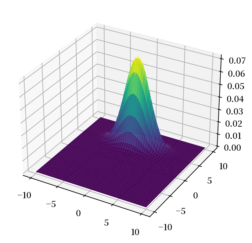
联合分布
让我们绘制总体联合密度。
# %matplotlib notebook

fig = plt.figure()
ax = plt.axes(projection='3d')

surf = ax.plot_surface(x_mesh, y_mesh, func(x_mesh, y_mesh), cmap='viridis')
plt.show()
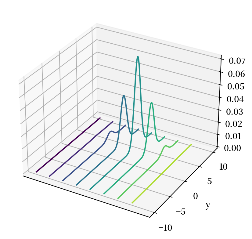
# %matplotlib notebook

fig = plt.figure()
ax = plt.axes(projection='3d')

curve = ax.contour(x_mesh, y_mesh, func(x_mesh, y_mesh), zdir='x')
plt.ylabel('y')
ax.set_zlabel('f')
ax.set_xticks([])
plt.show()
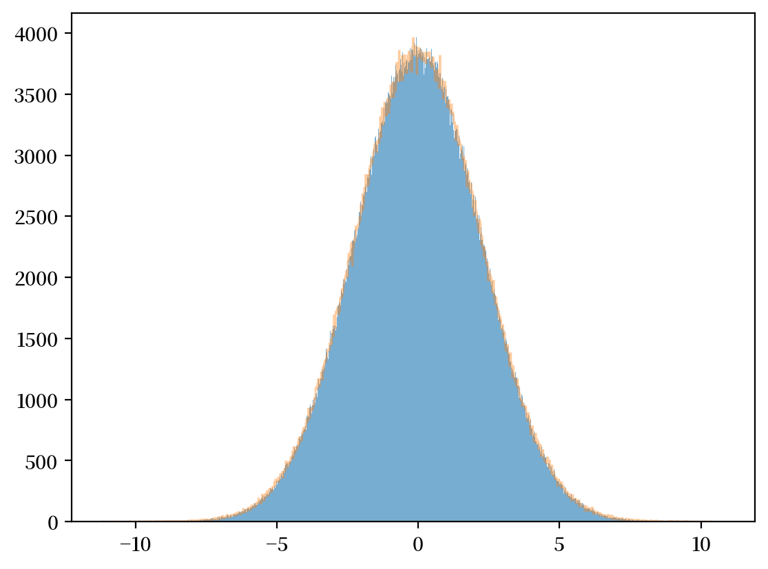
然后我们可以使用内置的numpy函数来进行模拟,并从样本均值和方差计算样本边际分布。
μ= np.array([0, 5])
σ= np.array([[5, .2], [.2, 1]])
n = 1_000_000
data = np.random.multivariate_normal(μ, σ, n)
x = data[:, 0]
y = data[:, 1]
边缘分布
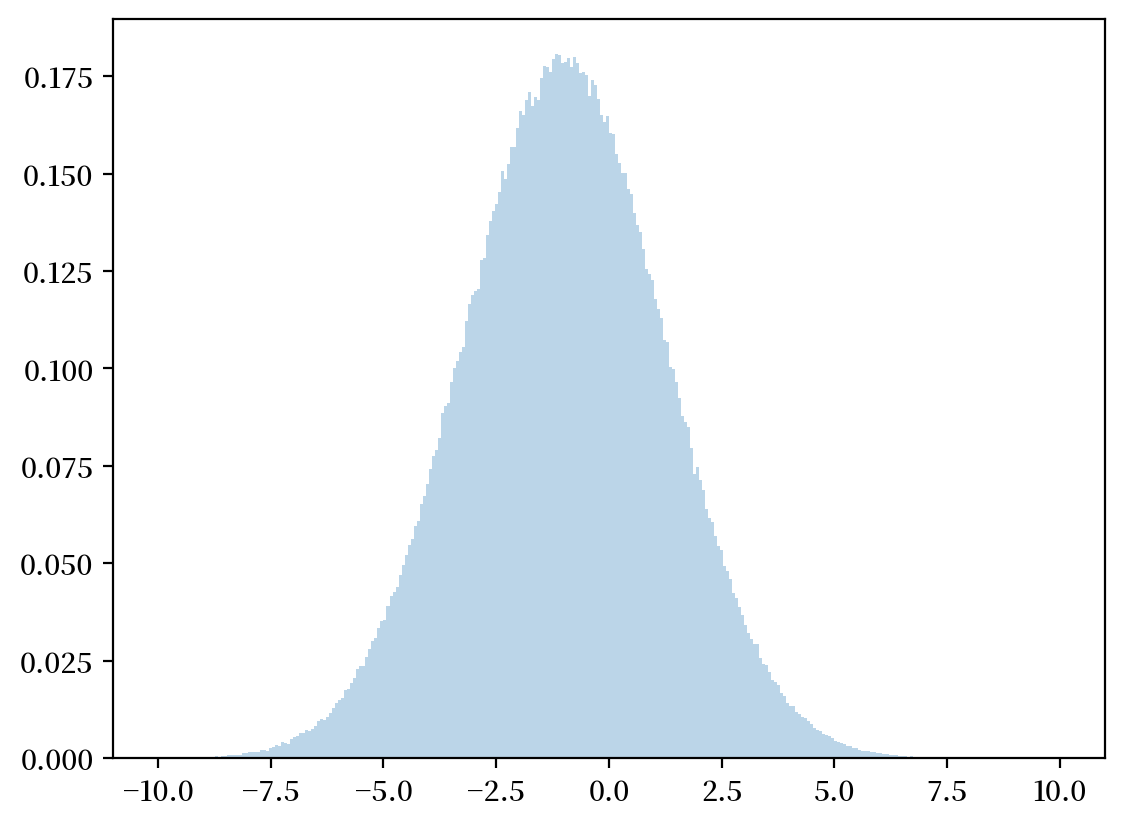
plt.hist(x, bins=1_000, alpha=0.6)
μx_hat, σx_hat = np.mean(x), np.std(x)
print(μx_hat, σx_hat)
x_sim = np.random.normal(μx_hat, σx_hat, 1_000_000)
plt.hist(x_sim, bins=1_000, alpha=0.4, histtype="step")
plt.show()
-0.00365252096577061 2.2402077440761747
plt.hist(y, bins=1_000, density=True, alpha=0.6)
μy_hat, σy_hat = np.mean(y), np.std(y)
print(μy_hat, σy_hat)
y_sim = np.random.normal(μy_hat, σy_hat, 1_000_000)
plt.hist(y_sim, bins=1_000, density=True, alpha=0.4, histtype="step")
plt.show()
4.999108836027072 0.9996132907308383

条件分布
对于二维正态(高斯)总体分布,其条件分布也服从正态分布:
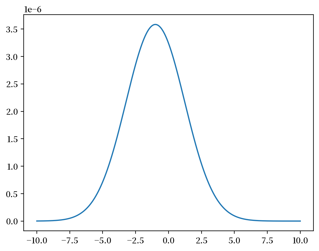
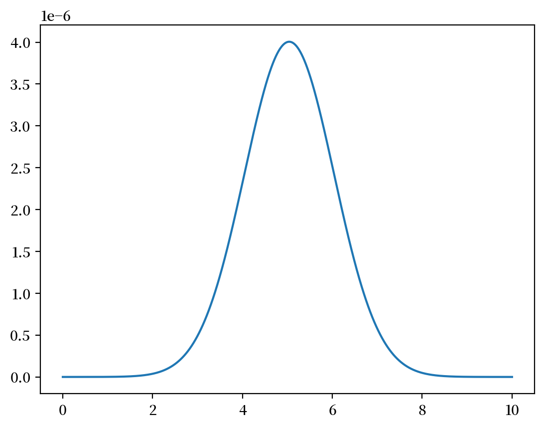
让我们通过离散化并将近似联合密度映射到矩阵中来近似联合密度。
我们可以通过使用矩阵代数并注意到以下关系来计算离散化边际密度:
固定 \(y=0\)。
# 离散化边际密度
x = np.linspace(-10, 10, 1_000_000)
z = func(x, y=0) / np.sum(func(x, y=0))
plt.plot(x, z)
plt.show()
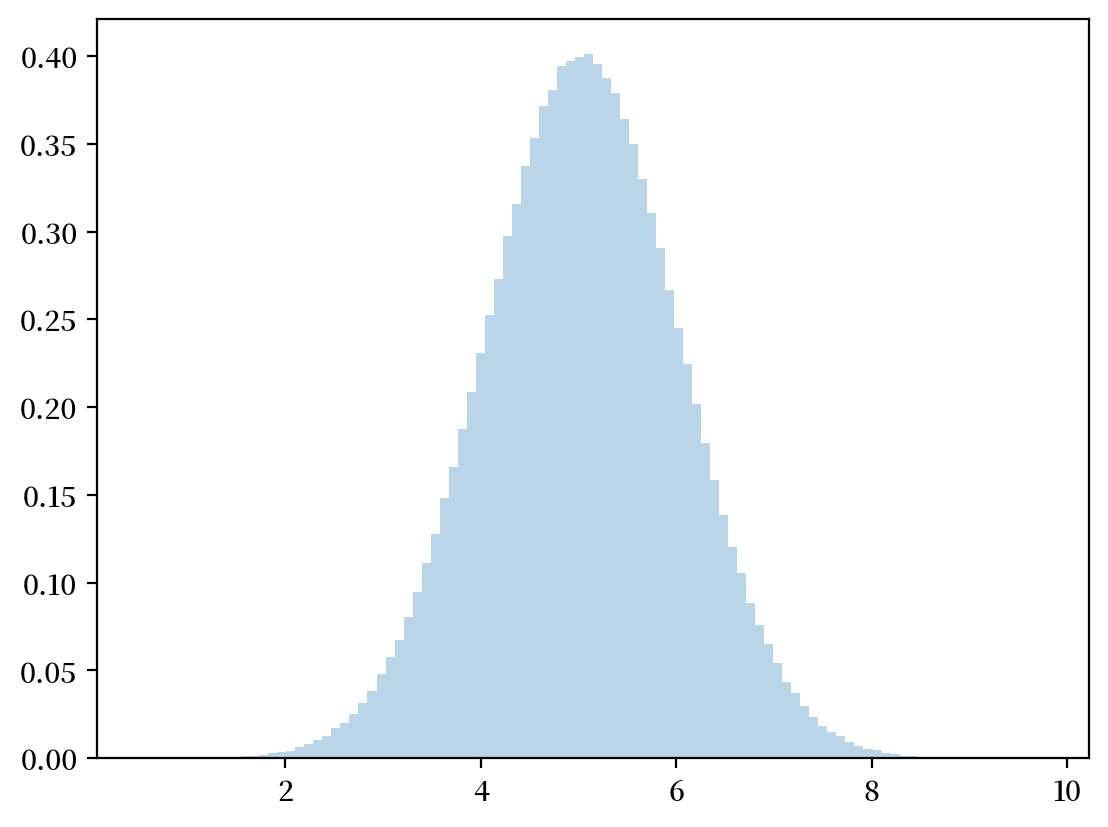
均值和方差的计算公式为
让我们从具有上述均值和方差的正态分布中采样,检验我们的近似值有多准确。
# 离散化均值
μx = np.dot(x, z)

# 离散化标准差
σx = np.sqrt(np.dot((x - μx)**2, z))

# 采样
zz = np.random.normal(μx, σx, 1_000_000)
plt.hist(zz, bins=300, density=True, alpha=0.3, range=[-10, 10])
plt.show()
固定 \(x=1\)。
y = np.linspace(0, 10, 1_000_000)
z = func(x=1, y=y) / np.sum(func(x=1, y=y))
plt.plot(y,z)
plt.show()
# 离散化的均值和标准差
μy = np.dot(y,z)
σy = np.sqrt(np.dot((y - μy)**2, z))

# 采样
zz = np.random.normal(μy,σy,1_000_000)
plt.hist(zz, bins=100, density=True, alpha=0.3)
plt.show()
我们将其与解析计算的参数进行比较,发现它们很接近。
print(μx, σx)
print(μ1 + ρ * σ1 * (0 - μ2) / σ2, np.sqrt(σ1**2 * (1 - ρ**2)))

print(μy, σy)
print(μ2 + ρ * σ2 * (1 - μ1) / σ1, np.sqrt(σ2**2 * (1 - ρ**2)))
-0.9997518414498469 2.226584133169768
-1.0 2.227105745132009
5.039999456960766 0.9959851265795594
5.04 0.9959919678390986
8.14. 两个独立分布随机变量的和#
设 \(X, Y\) 是两个独立的离散随机变量,分别取值于 \(\bar{X}, \bar{Y}\)。
定义一个新的随机变量 \(Z=X+Y\)。
显然,\(Z\) 取值于 \(\bar{Z}\),定义如下:
\(X\) 和 \(Y\) 的独立性意味着:
因此,我们有:
其中 \(f * g\) 表示序列 \(f\) 和 \(g\) 的卷积。
类似地,对于具有密度函数 \(f_{X}, g_{Y}\) 的两个随机变量 \(X,Y\),\(Z=X+Y\) 的密度函数为
其中 \( f_{X}*g_{Y} \) 表示函数 \(f_X\) 和 \(g_Y\) 的卷积。
考虑以下两个随机变量的联合概率分布。
设 \(X,Y\) 为离散随机变量,其联合分布为
其中 \(i = 0,\dots,I-1; j = 0,\dots,J-1\) 且
相关的条件分布为
我们可以定义转移概率矩阵
其中
第一行是在 \(X=0\) 条件下 \(Y=j, j=0,1\) 的概率。
第二行是在 \(X=1\) 条件下 \(Y=j, j=0,1\) 的概率。
注意
\(\sum_{j}\rho_{ij}= \frac{ \sum_{j}\rho_{ij}}{ \sum_{j}\rho_{ij}}=1\),所以 \(\rho\) 的每一行都是一个概率分布(每一列则不是)。
8.15. 耦合#
从联合分布开始
其中
从联合分布出发,我们已经证明可以得到唯一的边缘分布。
现在我们尝试反向推导。
我们会发现,从两个边缘分布出发,通常可以构造出多个满足这些边缘分布的联合分布。
这些联合分布中的每一个都被称为两个边缘分布的耦合。
让我们从边缘分布开始
给定两个边缘分布,\(X\)的分布\(\mu\)和\(Y\)的分布\(\nu\),联合分布\(f_{ij}\)被称为\(\mu\)和\(\nu\)的一个耦合。
例子:
考虑以下二元示例。
我们构造两个耦合。
这两个边缘分布的第一个耦合是以下联合分布:
为了验证这是一个耦合,我们检查
这两个边缘分布的第二个耦合是以下联合分布:
要验证这是一个耦合,注意到
因此,我们提出的两个联合分布具有相同的边际分布。
但是联合分布本身不同。
因此,多个联合分布 \([f_{ij}]\) 可以具有相同的边际分布。
注释:
耦合在最优传输问题和马尔可夫过程中很重要。
8.16. Copula函数#
假设 \(X_1, X_2, \dots, X_n\) 是 \(N\) 个随机变量,并且
它们的边际分布是 \(F_1(x_1), F_2(x_2),\dots, F_N(x_N)\),并且
它们的联合分布是\(H(x_1,x_2,\dots,x_N)\)
那么存在一个Copula函数\(C(\cdot)\)满足
我们可以得到
反过来,给定单变量边际分布\(F_1(x_1), F_2(x_2),\dots,F_N(x_N)\)和一个Copula函数\(C(\cdot)\),函数\(H(x_1,x_2,\dots,x_N) = C(F_1(x_1), F_2(x_2),\dots,F_N(x_N))\)是\(F_1(x_1), F_2(x_2),\dots,F_N(x_N)\)的一个耦合。
因此,对于给定的边际分布,当相关的单变量随机变量不独立时,我们可以使用Copula函数来确定联合分布。
Copula函数常被用来描述随机变量之间的相依性。
离散边际分布
如上所述,对于两个给定的边际分布,可能存在多个耦合。
例如,考虑两个随机变量 \(X, Y\) 的分布为
对于这两个随机变量,可能存在多个耦合。
让我们首先生成 X 和 Y。
# 定义参数
mu = np.array([0.6, 0.4])
nu = np.array([0.3, 0.7])

# 抽样次数
draws = 1_000_000

# 从均匀分布生成抽样
p = np.random.rand(draws)

# 通过均匀分布生成 X 和 Y 的抽样
x = np.ones(draws)
y = np.ones(draws)
x[p <= mu[0]] = 0
x[p > mu[0]] = 1
y[p <= nu[0]] = 0
y[p > nu[0]] = 1
# 从抽样中计算参数
q_hat = sum(x[x == 1])/draws
r_hat = sum(y[y == 1])/draws

# 打印输出
print("x的分布")
xmtb = pt.PrettyTable()
xmtb.field_names = ['x值', 'x概率']
xmtb.add_row([0, 1-q_hat])
xmtb.add_row([1, q_hat])
print(xmtb)

print("y的分布")
ymtb = pt.PrettyTable()
ymtb.field_names = ['y值', 'y概率']
ymtb.add_row([0, 1-r_hat])
ymtb.add_row([1, r_hat])
print(ymtb)
x的分布
+-----+----------+
| x值 |  x概率   |
+-----+----------+
|  0  | 0.599683 |
|  1  | 0.400317 |
+-----+----------+
y的分布
+-----+---------------------+
| y值 |        y概率        |
+-----+---------------------+
|  0  | 0.30013599999999996 |
|  1  |       0.699864      |
+-----+---------------------+
现在让我们用两个边际分布,一个是\(X\)的,另一个是\(Y\)的,来构造两个不同的耦合。
对于第一个联合分布:
其中
让我们使用Python来构造这个联合分布,然后验证其边际分布是否符合要求。
# 定义参数
f1 = np.array([[0.18, 0.42], [0.12, 0.28]])
f1_cum = np.cumsum(f1)

# 抽样次数
draws1 = 1_000_000

# 从均匀分布生成抽样
p = np.random.rand(draws1)

# 通过均匀分布生成第一个耦合的抽样
c1 = np.vstack([np.ones(draws1), np.ones(draws1)])
# X=0, Y=0
c1[0, p <= f1_cum[0]] = 0
c1[1, p <= f1_cum[0]] = 0
# X=0, Y=1
c1[0, (p > f1_cum[0])*(p <= f1_cum[1])] = 0
c1[1, (p > f1_cum[0])*(p <= f1_cum[1])] = 1
# X=1, Y=0
c1[0, (p > f1_cum[1])*(p <= f1_cum[2])] = 1
c1[1, (p > f1_cum[1])*(p <= f1_cum[2])] = 0
# X=1, Y=1
c1[0, (p > f1_cum[2])*(p <= f1_cum[3])] = 1
c1[1, (p > f1_cum[2])*(p <= f1_cum[3])] = 1
# 从抽样中计算参数
f1_00 = sum((c1[0, :] == 0)*(c1[1, :] == 0))/draws1
f1_01 = sum((c1[0, :] == 0)*(c1[1, :] == 1))/draws1
f1_10 = sum((c1[0, :] == 1)*(c1[1, :] == 0))/draws1
f1_11 = sum((c1[0, :] == 1)*(c1[1, :] == 1))/draws1

# 打印第一个联合分布
print("c1的第一个联合分布")
c1_mtb = pt.PrettyTable()
c1_mtb.field_names = ['c1_x值', 'c1_y值', 'c1概率']
c1_mtb.add_row([0, 0, f1_00])
c1_mtb.add_row([0, 1, f1_01])
c1_mtb.add_row([1, 0, f1_10])
c1_mtb.add_row([1, 1, f1_11])
print(c1_mtb)
c1的第一个联合分布
+--------+--------+----------+
| c1_x值 | c1_y值 |  c1概率  |
+--------+--------+----------+
|   0    |   0    | 0.179637 |
|   0    |   1    | 0.420967 |
|   1    |   0    | 0.11977  |
|   1    |   1    | 0.279626 |
+--------+--------+----------+
# 从抽样中计算参数
c1_q_hat = sum(c1[0, :] == 1)/draws1
c1_r_hat = sum(c1[1, :] == 1)/draws1

# 打印输出
print("x的边缘分布")
c1_x_mtb = pt.PrettyTable()
c1_x_mtb.field_names = ['c1_x_值', 'c1_x_概率']
c1_x_mtb.add_row([0, 1-c1_q_hat])
c1_x_mtb.add_row([1, c1_q_hat])
print(c1_x_mtb)

print("y的边缘分布")
c1_ymtb = pt.PrettyTable()
c1_ymtb.field_names = ['c1_y_值', 'c1_y_概率']
c1_ymtb.add_row([0, 1-c1_r_hat])
c1_ymtb.add_row([1, c1_r_hat])
print(c1_ymtb)
x的边缘分布
+---------+-----------+
| c1_x_值 | c1_x_概率 |
+---------+-----------+
|    0    |  0.600604 |
|    1    |  0.399396 |
+---------+-----------+
y的边缘分布
+---------+-----------+
| c1_y_值 | c1_y_概率 |
+---------+-----------+
|    0    |  0.299407 |
|    1    |  0.700593 |
+---------+-----------+
现在,让我们构造另一个也是 \(X\) 和 \(Y\) 的耦合的联合分布
# 定义参数
f2 = np.array([[0.3, 0.3], [0, 0.4]])
f2_cum = np.cumsum(f2)

# 抽样次数
draws2 = 1_000_000

# 从均匀分布生成抽样
p = np.random.rand(draws2)

# 通过均匀分布生成第一个耦合的抽样
c2 = np.vstack([np.ones(draws2), np.ones(draws2)])
# X=0, Y=0
c2[0, p <= f2_cum[0]] = 0
c2[1, p <= f2_cum[0]] = 0
# X=0, Y=1
c2[0, (p > f2_cum[0])*(p <= f2_cum[1])] = 0
c2[1, (p > f2_cum[0])*(p <= f2_cum[1])] = 1
# X=1, Y=0
c2[0, (p > f2_cum[1])*(p <= f2_cum[2])] = 1
c2[1, (p > f2_cum[1])*(p <= f2_cum[2])] = 0
# X=1, Y=1
c2[0, (p > f2_cum[2])*(p <= f2_cum[3])] = 1
c2[1, (p > f2_cum[2])*(p <= f2_cum[3])] = 1
# 从抽样中计算参数
f2_00 = sum((c2[0, :] == 0)*(c2[1, :] == 0))/draws2
f2_01 = sum((c2[0, :] == 0)*(c2[1, :] == 1))/draws2
f2_10 = sum((c2[0, :] == 1)*(c2[1, :] == 0))/draws2
f2_11 = sum((c2[0, :] == 1)*(c2[1, :] == 1))/draws2

# 打印第二个联合分布的输出
print("c2的第一个联合分布")
c2_mtb = pt.PrettyTable()
c2_mtb.field_names = ['c2_x值', 'c2_y值', 'c2_概率']
c2_mtb.add_row([0, 0, f2_00])
c2_mtb.add_row([0, 1, f2_01])
c2_mtb.add_row([1, 0, f2_10])
c2_mtb.add_row([1, 1, f2_11])
print(c2_mtb)
c2的第一个联合分布
+--------+--------+----------+
| c2_x值 | c2_y值 | c2_概率  |
+--------+--------+----------+
|   0    |   0    | 0.300442 |
|   0    |   1    | 0.300024 |
|   1    |   0    |   0.0    |
|   1    |   1    | 0.399534 |
+--------+--------+----------+
# 从抽样中计算参数
c2_q_hat = sum(c2[0, :] == 1)/draws2
c2_r_hat = sum(c2[1, :] == 1)/draws2

# 打印输出
print("x的边缘分布")
c2_x_mtb = pt.PrettyTable()
c2_x_mtb.field_names = ['c2_x_取值', 'c2_x_概率']
c2_x_mtb.add_row([0, 1-c2_q_hat])
c2_x_mtb.add_row([1, c2_q_hat])
print(c2_x_mtb)

print("y的边缘分布")
c2_ymtb = pt.PrettyTable()
c2_ymtb.field_names = ['c2_y_取值', 'c2_y_概率']
c2_ymtb.add_row([0, 1-c2_r_hat])
c2_ymtb.add_row([1, c2_r_hat])
print(c2_ymtb)
x的边缘分布
+-----------+--------------------+
| c2_x_取值 |     c2_x_概率      |
+-----------+--------------------+
|     0     | 0.6004659999999999 |
|     1     |      0.399534      |
+-----------+--------------------+
y的边缘分布
+-----------+-----------+
| c2_y_取值 | c2_y_概率 |
+-----------+-----------+
|     0     |  0.300442 |
|     1     |  0.699558 |
+-----------+-----------+
经过验证,联合分布 \(c_1\) 和 \(c_2\) 具有相同的 \(X\) 和 \(Y\) 的边际分布。
因此它们都是 \(X\) 和 \(Y\) 的耦合。