41. 卡尔曼滤波器进阶#
在之前的量化经济学讲座 卡尔曼滤波器的初步介绍 中,我们使用卡尔曼滤波器来估计火箭的位置。
在本讲座中,我们将使用卡尔曼滤波器来推断劳动者的:
人力资本
劳动者投入人力资本积累的努力程度
这两个变量都是公司无法直接观察到的。
公司只能通过观察劳动者历史产出,以及理解这些产出如何依赖于劳动者的人力资本,以及人力资本如何作为劳动者努力程度的函数来演化,来了解上述变量。
我们将设定一个规则,说明公司如何根据每期获得的信息来支付劳动者工资。
除了Anaconda中的内容外,本讲座还需要以下库:
!pip install quantecon
为了进行模拟,我们引入以下函数库,与 卡尔曼滤波器的初步介绍 相同:
import matplotlib.pyplot as plt
import matplotlib as mpl
FONTPATH = "fonts/SourceHanSerifSC-SemiBold.otf"
mpl.font_manager.fontManager.addfont(FONTPATH)
plt.rcParams['font.family'] = ['Source Han Serif SC']

import numpy as np
from quantecon import Kalman, LinearStateSpace
from collections import namedtuple
from scipy.stats import multivariate_normal
import matplotlib as mpl

# Configure Matplotlib to use pdfLaTeX and CJKutf8
mpl.rcParams.update({
    'text.usetex': True,
    'text.latex.preamble': r'''
        \usepackage{{CJKutf8}}
        \usepackage{{amsmath}}
    '''
})

# Function to wrap Chinese text in CJK environment
def cjk(text):
    return rf'\begin{{CJK}}{{UTF8}}{{gbsn}}{text}\end{{CJK}}'
41.1. 劳动者的产出#
一个代表性劳动者永久受雇于一家公司。
劳动者的产出由以下动态过程描述:
其中:
\(h_t\) 是时间 \(t\) 时的人力资本对数
\(u_t\) 是时间 \(t\) 时劳动者投入人力资本积累的努力程度的对数
\(y_t\) 是时间 \(t\) 时劳动者产出的对数
\(h_0 \sim {N}(\hat h_0, \sigma_{h,0})\)
\(u_0 \sim {N}(\hat u_0, \sigma_{u,0})\)
模型的参数包括 \(\alpha, \beta, c, R, g, \hat h_0, \hat u_0, \sigma_h, \sigma_u\)。
在时间 \(0\),公司雇佣了劳动者。
劳动者永久依附于公司,因此在所有时间 \(t =0, 1, 2, \ldots\) 都为同一家公司工作。
在时间 \(0\) 开始时,公司既无法观察到劳动者的初始人力资本 \(h_0\),也无法观察到其固有的永久努力水平 \(u_0\)。
公司认为特定劳动者的 \(u_0\) 服从高斯概率分布,因此由 \(u_0 \sim {N}(\hat u_0, \sigma_{u,0})\) 描述。
劳动者”类型”中的 \(h_t\) 部分随时间变化,但努力程度部分 \(u_t = u_0\) 保持不变。
这意味着从公司的角度来看,劳动者的努力程度实际上是一个未知的固定”参数”。
在任意时间点 \(t\geq 1\),公司能观察到该劳动者从雇佣开始到当前时刻的所有历史产出记录,记为 \(y^{t-1} = [y_{t-1}, y_{t-2}, \ldots, y_0]\)。
虽然公司无法直接观察劳动者的真实”类型”(即初始人力资本 \(h_0\) 和固有努力水平 \(u_0\)),但可以通过观察劳动者当前的产出 \(y_t\) 以及回顾其历史产出记录 \(y^{t-1}\) 来进行推断。
41.2. 公司的工资设定政策#
公司根据掌握的劳动者信息来确定工资。具体来说:
对于 \(t \geq 1\) 时期,公司基于截至 \(t-1\) 时期的产出历史 \(y^{t-1}\) 来预测劳动者当前的人力资本水平 \(h_t\)。劳动者的对数工资设定为:
而在初始时期 \(t=0\),由于还没有任何历史信息,公司只能基于先验均值来设定工资:
这种工资设定方式考虑到了一个事实:劳动者的实际产出中包含一个纯随机的成分 \(v_t\)。这个随机成分与劳动者的人力资本 \(h_t\) 和努力水平 \(u_t\) 都是相互独立的。
41.3. 状态空间表示#
将系统 (41.1) 写成状态空间形式:
这等价于:
其中:
为了计算公司的工资设定政策,我们首先创建一个 namedtuple 来存储模型的参数:
WorkerModel = namedtuple("WorkerModel",
                ('A', 'C', 'G', 'R', 'xhat_0', 'Σ_0'))

def create_worker(α=.8, β=.2, c=.2,
                  R=.5, g=1.0, hhat_0=4, uhat_0=4,
                  σ_h=4, σ_u=4):

    A = np.array([[α, β],
                  [0, 1]])
    C = np.array([[c],
                  [0]])
    G = np.array([g, 1])

    # 定义初始状态和协方差矩阵
    xhat_0 = np.array([[hhat_0],
                       [uhat_0]])

    Σ_0 = np.array([[σ_h, 0],
                    [0, σ_u]])

    return WorkerModel(A=A, C=C, G=G, R=R, xhat_0=xhat_0, Σ_0=Σ_0)
WorkerModel namedtuple 为我们创建了所有需要的对象,以便构建状态空间表示 (41.2)。
这使得我们能够方便地使用 LinearStateSpace 类来模拟劳动者的历史 \(\{y_t, h_t\}\)。
# 定义 A, C, G, R, xhat_0, Σ_0
worker = create_worker()
A, C, G, R = worker.A, worker.C, worker.G, worker.R
xhat_0, Σ_0 = worker.xhat_0, worker.Σ_0

# 创建 LinearStateSpace 对象
ss = LinearStateSpace(A, C, G, np.sqrt(R),
        mu_0=xhat_0, Sigma_0=np.zeros((2,2)))

T = 100
x, y = ss.simulate(T)
y = y.flatten()

h_0, u_0 = x[0, 0], x[1, 0]
接下来,为了计算公司基于其获得的关于劳动者的信息来设定对数工资的政策,我们使用本量化经济学讲座 卡尔曼滤波器的初步介绍 中描述的卡尔曼滤波器。
特别是,我们想要计算”创新表示”中的所有对象。
41.4. 创新表示#
我们已经掌握了形成劳动者产出过程 \(\{y_t\}_{t=0}^T\) 的创新表示所需的所有对象。
让我们现在编写代码:
其中 \(K_t\) 是时间 \(t\) 的卡尔曼增益矩阵。
我们使用 Kalman 类来完成这个任务:
kalman = Kalman(ss, xhat_0, Σ_0)
Σ_t = np.zeros((*Σ_0.shape, T-1))
y_hat_t = np.zeros(T-1)
x_hat_t = np.zeros((2, T-1))

for t in range(1, T):
    kalman.update(y[t])
    x_hat, Σ = kalman.x_hat, kalman.Sigma
    Σ_t[:, :, t-1] = Σ
    x_hat_t[:, t-1] = x_hat.reshape(-1)
    [y_hat_t[t-1]] = worker.G @ x_hat

x_hat_t = np.concatenate((x[:, 1][:, np.newaxis],
                    x_hat_t), axis=1)
Σ_t = np.concatenate((worker.Σ_0[:, :, np.newaxis],
                    Σ_t), axis=2)
u_hat_t = x_hat_t[1, :]
对于 \(h_0, u_0\) 的一个实现,我们绘制 \(E y_t = G \hat x_t \),其中 \(\hat x_t = E [x_t | y^{t-1}]\)。
我们还绘制 \(E [u_0 | y^{t-1}]\),这是公司基于其拥有的信息 \(y^{t-1}\) 对劳动者固有的”工作努力程度” \(u_0\) 的推断。
我们可以观察公司对劳动者工作努力程度的推断 \(E [u_0 | y^{t-1}]\) 如何逐渐收敛于隐藏的 \(u_0\),而 \(u_0\) 是公司无法直接观察到的。
fig, ax = plt.subplots(1, 2)

ax[0].plot(y_hat_t, label=r'$E[y_t| y^{t-1}]$')
ax[0].set_xlabel(cjk('时间'))
ax[0].set_ylabel(r'$E[y_t]$')
ax[0].set_title(cjk('$E[y_t]$ 随时间变化'))
ax[0].legend()

ax[1].plot(u_hat_t, label=r'$E[u_t|y^{t-1}]$')
ax[1].axhline(y=u_0, color='grey',
            linestyle='dashed', label=fr'$u_0={u_0:.2f}$')
ax[1].set_xlabel(cjk('时间'))
ax[1].set_ylabel(r'$E[u_t|y^{t-1}]$')
ax[1].set_title(cjk('推断的工作伦理随时间变化'))
ax[1].legend()

fig.tight_layout()
plt.show()

41.5. 一些计算实验#
让我们看看 \(\Sigma_0\) 和 \(\Sigma_T\),以表示公司在设定的时间范围内对隐藏状态了解多少。
print(Σ_t[:, :, 0])
[[4. 0.]
 [0. 4.]]
print(Σ_t[:, :, -1])
[[0.08805027 0.00100377]
 [0.00100377 0.00398351]]
显然,条件协方差矩阵中的元素随时间变小。
通过在不同时间 \(t\) 绘制 \(E [x_t |y^{t-1}] \) 周围的置信椭圆,我们可以形象地展示条件协方差矩阵 \(\Sigma_t\) 如何演化。
# 创建用于等高线绘制的点网格
h_range = np.linspace(x_hat_t[0, :].min()-0.5*Σ_t[0, 0, 1],
                      x_hat_t[0, :].max()+0.5*Σ_t[0, 0, 1], 100)
u_range = np.linspace(x_hat_t[1, :].min()-0.5*Σ_t[1, 1, 1],
                      x_hat_t[1, :].max()+0.5*Σ_t[1, 1, 1], 100)
h, u = np.meshgrid(h_range, u_range)

# 为每个时间步创建子图
fig, axs = plt.subplots(1, 3, figsize=(12, 7))

# 遍历每个时间步
for i, t in enumerate(np.linspace(0, T-1, 3, dtype=int)):
    # 创建具有时间步 t 的 x_hat 和 Σ 的多变量正态分布
    mu = x_hat_t[:, t]
    cov = Σ_t[:, :, t]
    mvn = multivariate_normal(mean=mu, cov=cov)

    # 在网格上评估多变量正态 PDF
    pdf_values = mvn.pdf(np.dstack((h, u)))

    # 创建 PDF 的等高线图
    con = axs[i].contour(h, u, pdf_values, cmap='viridis')
    axs[i].clabel(con, inline=1, fontsize=10)
    axs[i].set_title(cjk('时间步')+f'{t+1}')
    axs[i].set_xlabel(r'$h_{{{}}}$'.format(str(t+1)))
    axs[i].set_ylabel(r'$u_{{{}}}$'.format(str(t+1)))

    cov_latex = r'$\Sigma_{{{}}}= \begin{{bmatrix}} {:.2f} & {:.2f} \\ {:.2f} & {:.2f} \end{{bmatrix}}$'.format(
        t+1, cov[0, 0], cov[0, 1], cov[1, 0], cov[1, 1]
    )
    axs[i].text(0.33, -0.15, cov_latex, transform=axs[i].transAxes)


plt.tight_layout()
plt.show()
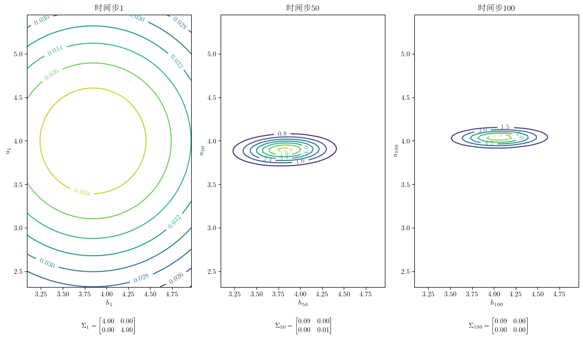
注意 \(y^t\) 的积累是如何随着样本量 \(t\) 的增长影响置信椭圆的形状。
现在让我们使用我们的代码将隐藏状态 \(x_0\) 设置为特定的向量,以观察公司如何从我们感兴趣的某个 \(x_0\) 开始学习。
例如,让我们设 \(h_0 = 0\) 和 \(u_0 = 4\)。
这是实现这个例子的一种方式:
# 例如,我们可能想要 h_0 = 0 和 u_0 = 4
mu_0 = np.array([0.0, 4.0])

# 创建一个 LinearStateSpace 对象,其中 Sigma_0 为零矩阵
ss_example = LinearStateSpace(A, C, G, np.sqrt(R), mu_0=mu_0,
                              # 这行强制 h_0=0 和 u_0=4
                              Sigma_0=np.zeros((2, 2))
                             )

T = 100
x, y = ss_example.simulate(T)
y = y.flatten()

# 现在 h_0=0 和 u_0=4
h_0, u_0 = x[0, 0], x[1, 0]
print('h_0 =', h_0)
print('u_0 =', u_0)
h_0 = 0.0
u_0 = 4.0
实现相同例子的另一种方式是使用以下代码:
# 如果我们想要设置初始
# h_0 = hhat_0 = 0 和 u_0 = uhhat_0 = 4.0:
worker = create_worker(hhat_0=0.0, uhat_0=4.0)

ss_example = LinearStateSpace(A, C, G, np.sqrt(R),
                              # 这行取 h_0=hhat_0 和 u_0=uhhat_0
                              mu_0=worker.xhat_0,
                              # 这行强制 h_0=hhat_0 和 u_0=uhhat_0
                              Sigma_0=np.zeros((2, 2))
                             )

T = 100
x, y = ss_example.simulate(T)
y = y.flatten()

# 现在 h_0 和 u_0 将精确等于 hhat_0
h_0, u_0 = x[0, 0], x[1, 0]
print('h_0 =', h_0)
print('u_0 =', u_0)
h_0 = 0.0
u_0 = 4.0
对于这个劳动者,让我们生成一个类似上面的图:
# 首先我们使用初始 xhat_0 和 Σ_0 计算卡尔曼滤波器
kalman = Kalman(ss, xhat_0, Σ_0)
Σ_t = []
y_hat_t = np.zeros(T-1)
u_hat_t = np.zeros(T-1)

# 然后我们使用基于上述线性状态模型的观测值 y
# 迭代更新卡尔曼滤波器类:
for t in range(1, T):
    kalman.update(y[t])
    x_hat, Σ = kalman.x_hat, kalman.Sigma
    Σ_t.append(Σ)
    [y_hat_t[t-1]] = worker.G @ x_hat
    [u_hat_t[t-1]] = x_hat[1]


# 生成 y_hat_t 和 u_hat_t 的图
fig, ax = plt.subplots(1, 2)

ax[0].plot(y_hat_t, label=r'$E[y_t| y^{t-1}]$')
ax[0].set_xlabel(cjk('时间'))
ax[0].set_ylabel(r'$E[y_t]$')
ax[0].set_title(cjk('$E[y_t]$ 随时间变化'))
ax[0].legend()

ax[1].plot(u_hat_t, label=r'$E[u_t|y^{t-1}]$')
ax[1].axhline(y=u_0, color='grey',
            linestyle='dashed', label=fr'$u_0={u_0:.2f}$')
ax[1].set_xlabel(cjk('时间'))
ax[1].set_ylabel(r'$E[u_t|y^{t-1}]$')
ax[1].set_title(cjk('推断的工作伦理随时间变化'))
ax[1].legend()

fig.tight_layout()
plt.show()

更一般地,我们可以在 create_worker namedtuple 中更改定义劳动者的部分或全部参数。
这是一个例子:
# 我们可以在创建劳动者时设置这些参数 -- 就像类一样!
hard_working_worker =  create_worker(α=.4, β=.8,
                        hhat_0=7.0, uhat_0=100, σ_h=2.5, σ_u=3.2)

print(hard_working_worker)
WorkerModel(A=array([[0.4, 0.8],
       [0. , 1. ]]), C=array([[0.2],
       [0. ]]), G=array([1., 1.]), R=0.5, xhat_0=array([[  7.],
       [100.]]), Σ_0=array([[2.5, 0. ],
       [0. , 3.2]]))
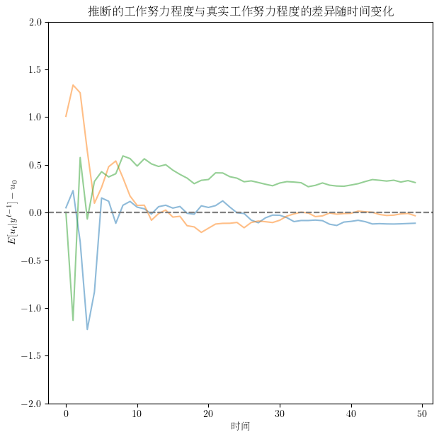
让我们通过模拟不同劳动者在50个时期内的表现来进一步理解这个系统。
有趣的是,我们会发现随着时间推移,公司对劳动者真实努力程度的估计会越来越准确 - 估计值和实际值之间的差异会逐渐趋近于零。
这说明卡尔曼滤波器在帮助公司和劳动者之间建立信息沟通的桥梁,使公司对劳动者真实努力程度的估计越来越准确。
num_workers = 3
T = 50
fig, ax = plt.subplots(figsize=(7, 7))

for i in range(num_workers):
    worker = create_worker(uhat_0=4+2*i)
    simulate_workers(worker, T, ax)
ax.set_ylim(ymin=-2, ymax=2)
plt.show()
# 我们还可以生成 u_t 的图:

T = 50
fig, ax = plt.subplots(figsize=(7, 7))

uhat_0s = [2, -2, 1]
αs = [0.2, 0.3, 0.5]
βs = [0.1, 0.9, 0.3]

for i, (uhat_0, α, β) in enumerate(zip(uhat_0s, αs, βs)):
    worker = create_worker(uhat_0=uhat_0, α=α, β=β)
    simulate_workers(worker, T, ax,
                    # 通过设置 diff=False,它将给出 u_t
                    diff=False, name=r'$u_{{{}, t}}$'.format(i))

ax.axhline(y=u_0, xmin=0, xmax=0, color='grey',
           linestyle='dashed', label=r'$u_{i, 0}$')
ax.legend(bbox_to_anchor=(1, 0.5))
plt.show()

# 我们还可以为所有劳动者使用精确的 u_0=1 和 h_0=2

T = 50
fig, ax = plt.subplots(figsize=(7, 7))

# 这两行设置所有劳动者的 u_0=1 和 h_0=2
mu_0 = np.array([[1],
                 [2]])
Sigma_0 = np.zeros((2,2))

uhat_0s = [2, -2, 1]
αs = [0.2, 0.3, 0.5]
βs = [0.1, 0.9, 0.3]

for i, (uhat_0, α, β) in enumerate(zip(uhat_0s, αs, βs)):
    worker = create_worker(uhat_0=uhat_0, α=α, β=β)
    simulate_workers(worker, T, ax, mu_0=mu_0, Sigma_0=Sigma_0,
                     diff=False, name=r'$u_{{{}, t}}$'.format(i))

# 这控制图的边界
ax.set_ylim(ymin=-3, ymax=3)
ax.axhline(y=u_0, xmin=0, xmax=0, color='grey',
           linestyle='dashed', label=r'$u_{i, 0}$')
ax.legend(bbox_to_anchor=(1, 0.5))
plt.show()

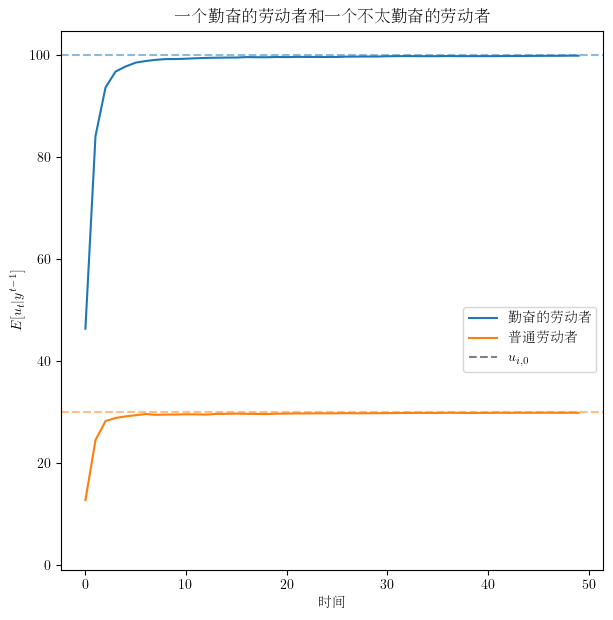
# 我们可以只为其中一个劳动者生成图:

T = 50
fig, ax = plt.subplots(figsize=(7, 7))

mu_0_1 = np.array([[1],
                 [100]])
mu_0_2 = np.array([[1],
                 [30]])
Sigma_0 = np.zeros((2,2))

uhat_0s = 100
αs = 0.5
βs = 0.3

worker = create_worker(uhat_0=uhat_0, α=α, β=β)
simulate_workers(worker, T, ax, mu_0=mu_0_1, Sigma_0=Sigma_0,
                 diff=False, name=cjk('勤奋的劳动者'))
simulate_workers(worker, T, ax, mu_0=mu_0_2, Sigma_0=Sigma_0,
                 diff=False,
                 title=cjk('一个勤奋的劳动者和一个不太勤奋的劳动者'),
                 name=cjk('普通劳动者'))
ax.axhline(y=u_0, xmin=0, xmax=0, color='grey',
           linestyle='dashed', label=r'$u_{i, 0}$')
ax.legend(bbox_to_anchor=(1, 0.5))
plt.show()
41.6. 未来扩展#
我们可以进行许多有趣的实验,比如创建不同类型的劳动者,让公司通过观察他们的产出历史来推断他们的隐藏特征(如能力和努力程度)。这种设置可以帮助我们理解信息不对称下的劳动力市场动态。